Brain Tumor Classification Using Back Propagation Neural Network

Early detection and classification of brain tumors is very important in clinical practice. Many researchers have proposed different techniques for the classification of brain tumors based on different sources of information. In this paper we propose a process for brain tumor classification, focusing on the analysis of Magnetic Resonance (MR) images data collected with benign and malignant tumors. Our aim is to achieve a high accuracy in discriminating the two types of tumors through a combination of several techniques such as image processing, feature extraction and classification. The proposed technique has the potential of assisting clinical diagnosis.

Image processing techniques are playing important role in analysing anatomical structures of human body. Image acquisition techniques like magnetic resonance imaging (MRI), X-Ray, ultrasound, mammography, CT-scan are highly dependent on computer technology to generate digital images. After obtaining digital images, image processing techniques can be further used for analysis of region of interest.

A tumor is a mass of tissue that serves no useful purpose and generally exists at the expense of healthy tissues. Malignant brain tumors do not have distinct borders. They tend to grow rapidly, increasing pressure within the brain and can spread in the brain or spinal cord beyond the point where they originate. They grow faster than benign tumors and are more likely to cause health problems.

Benign brain tumors, composed of harmless cells, have clearly defined borders, can usually be completely removed and are unlikely to recur. A benign tumor is basically a tumor that doesn't come back and doesn't spread to other parts of the body. Benign tumors tend to grow more slowly than malignant tumors and are less likely to cause health problems. In brain MR images, after appropriate segmentation of brain tumor classification of tumor in to malignant and benign is difficult task due to complexity and variations in tumor tissue characteristics like its shape, size, gray level intensities and location [1].

Feature extraction is an important issue for any pattern recognition problem. Most of the reported work is dedicated to tumor segmentation or tumor detection [1-6]. This paper presents a hybrid approach to classify malignant and benign tumors using some prior knowledge like pixel intensity and some anatomical features are proposed. MATLAB ® 7.01, its image processing toolbox is used for feature extraction and ANN toolbox has been used for classification.

The overall organization of the paper is as follows. The steps used to extract the principal features using Principal component analysis are explained in Section II. Section III describes the proposed methodology used and in each subsection it has been explained in details. Section IV demonstrates some simulation results and their performance evaluation finally conclusions are presented in section VI which tells the advantages of this work. Some other future works in this field has been proposed in this part too.

• II.    FEATURE EXTRACTION USING PRINCIPAL COMPONENT ANALYSIS (PCA)

In this paper, the principal component analysis (PCA) is used as a feature extraction algorithm. The principal component analysis (PCA) is one of the most successful techniques that have been used in image recognition and compression. The purpose of PCA is to reduce the large dimensionality of the data. Instead of employing all of the features, a preprocessing step of feature selection is performed using PCA aiming to remove the redundant features. Based on the statistical information, only the most informative features extracted from the MR images are utilized in the process.

The steps used to extract the principal components using principal component analysis are as follows:

• 1.    Convert the 2D images into one dimensional image using reshape function for both test image and database images.

• 2.    Find the mean value for each one dimensional image by dividing sum of pixel values and number of pixel values.

• 3.    Find the difference matrix for each images by [A] = (Original pixel intensity of 1D image) – (mean value).

• 4.    Find the covariance matrix by, covariance(L)=A *A^’

• 5.    Find the Eigen vector for 1D image by, [V D] = eig (L)

• 6.    Find the Eigen face of 1D image by, Eigen face = Eigen vector * A

By using this statement, we can get the Vector and diagonal matrix of the 1D image.

By using this principal component, we can identify the image from database which is similar to the features of test image.

One of the most common forms of dimensionality reduction is principal components analysis. Given a set of data, PCA finds the linear lower-dimensional representation of the data such that the variance of the reconstructed data is preserved. Using a system of feature reduction based on a combined principle component analysis on the feature lead to an efficient classification algorithm utilizing supervised approach. So, the main idea behind using PCA in our approach is to reduce the dimensionality and this leads to more efficient and accurate classifier.

PCA is a mathematical procedure that uses an orthogonal transformation to convert a set of observations of possibly correlated variables into a set of values of linearly uncorrelated variables called principal components . The number of principal components is less than or equal to the number of original variables. This transformation is defined in such a way that the first principal component has the largest possible variance (that is, accounts for as much of the variability in the data as possible), and each succeeding component in turn has the highest variance possible under the constraint that it be orthogonal to (i.e., uncorrelated with) the preceding components. Principal components are guaranteed to be independent only if the data set is jointly normally distributed. PCA is sensitive to the relative scaling of the original variables. Depending on the field of application, it is also named the discrete Karhunen–Loève transform (KLT), the Hotelling transform or proper orthogonal decomposition (POD) . It is mostly used as a tool in exploratory data analysis and for making predictive models.

The first principal component is the combination of variables that explains the greatest amount of variation. The second principal component defines the next largest amount of variation and is independent to the first principal component. There can be as many possible principal components as there are variables. It can be viewed as a rotation of the existing axes to new positions in them space defined by the original variables. In this new rotation, there will be no correlation between the new variables defined by the rotation. The first new variable contains the maximum amount of variation; the second new variable contains the maximum amount of variation unexplained by the first and orthogonal to the first, etc.

It can be viewed as finding a projection of the observations onto orthogonal axes contained in the space defined by the original variables. The criteria being that the first axis "contains " the maximum amount of variation, or "accounts" for the maximum amount of variation. The second axis contains the maximum amount of variation orthogonal to the first. The third axis contains the maximum amount of variation orthogonal to the first and second axis and so on until one has the last new axis which is the last amount of variation left.

PCA can be done by eigenvalue decomposition of a data covariance (or correlation) matrix or singular value decomposition of a data matrix, usually after mean centering (and normalizing or using Z-scores) the data matrix for each attribute. The results of a PCA are usually discussed in terms of component scores, sometimes called factor scores (the transformed variable values corresponding to a particular data point), and loadings (the weight by which each standardized original variable should be multiplied to get the component score [7].

• III.    PROPOSED METHODOLOGY

• A.    Database Preparation

The brain MRI images consisting of malignant and benign tumors were collected from open source database and some hospitals. Figure 1, shows some sample images from the database.

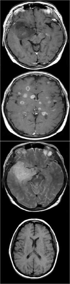
Figure.1 Example images from the Database

• B.    Calculation of Feature Vector

Feature extraction is the main aspect of any system. The feature vector of each image in the database is stored as .mat file. In the training phase, feature vectors are extracted for each image in the training set. Let Ω1 be a training image of image 1 which has a pixel resolution of M x N (M rows, N columns). In order to extract PCA features of Ω1, first convert the image into a pixel vector Φ1 by concatenating each of the M rows into a single vector. The length (or, dimensionality) of the vector Φ1 will be M x N. In this paper, the PCA algorithm is used as a dimensionality reduction technique which transforms the vector Φ1 to a vector ω1 which has a dimensionality d where d << M x N. For each training image Ωi, these feature vectors ωi are calculated and stored.

In the testing phase, the feature vector ωj of the test image Ωj is computed using PCA. In order to identify the test image Ωj, the similarities between ωj and all of the feature vectors ωi’s in the training set are computed. The similarity between feature vectors is computed using Euclidean distance. The identity of the most similar ωi is the output of the image recognizer. If i = j , it means that the MR image j has correctly identified, otherwise if i ≠ j , it means that the MR image j has misclassified. Schematic diagram of the MR image recognition system is shown in figure 2.

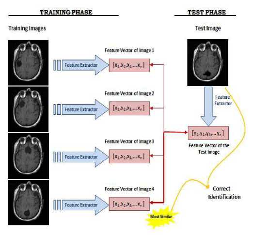
Figure.2 Schematic diagram of a MR image recognizer

• C.    Classification Using Back Propagation Algorithm

In this back-propagation algorithm is finally used for classifying the pattern of malignant and benign tumor. A three layer Neural network was created with 15 nodes in the first (input) layer, 1 to 15 nodes in the hidden layer, and 1 node as the output layer. We varied the number of nodes in the hidden layer in a simulation in order to determine the optimal number of hidden nodes. The back-propagation learning rule can be used to adjust the weights and biases of networks to minimize the sum squared error of the network [9, 10]. The activation function considered for each node in the network is the binary sigmoidal function defined (with s

= 1) as output = 1/ (1+e-x), where x is the sum of the weighted inputs to that particular node. This is a common function used in many BPN. This function limits the output of all nodes in the network to be between 0 and 1. Neural networks are basically trained until the error for each training iteration stops decreasing. A feature vector of each image in the database was generated and saved as in .mat file in MATLAB environment. 50% of the data has been used for training and remaining 50% was used for testing and validation.

• D.    Methodology

Back propagation neural network had been used for classification problems. The BPN classifier presented good accuracy, very small training time, robustness to weight changes.

There are 6 stages involved in the proposed model which are starting from the data input to output. The first stage should be the image processing system. Basically in image processing system, image acquisition and image enhancement are the steps that have to be done. In this paper, these two steps are skipped and all the images are collected from available resource. The proposed model requires converting the image into a format capable of being manipulated by the computer. The MR images are converted into matrices form by using MATLAB. Then, the BPN is used to classify the MR images. Lastly, performance based on the result will be analyzed at the end of the development phase. The proposed brain MR images classification method is shown in figure 3.

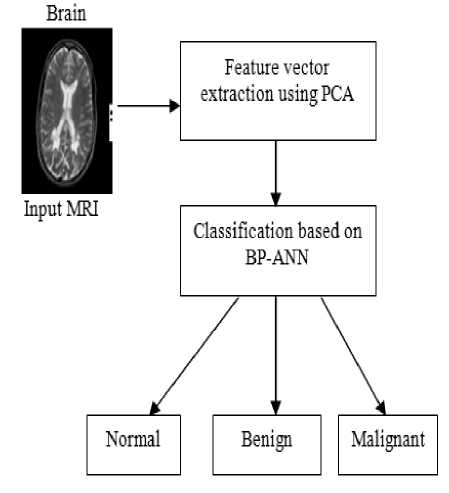
Figure.3 Proposed Model

• IV.    EXPERIMENT SIMULATION AND RESULT

Various experiments were performed and the training and the testing sets were determined by taking into consideration the classification accuracies. The data set was divided into two separate data sets – the training data set and the testing data set. The training data set was used to train the network, whereas the testing data set was used to verify the accuracy and the effectiveness of the trained network for the classification of brain tumors. The proposed technique is implemented in the working platform MATLAB and it is evaluated using 15 medical brain MRI images, which are collected from open source database and some hospitals. Among 15 MRI images, 5 images are normal, 5 images are benign tumor and the remaining of malignant tumor. The figure 1, shows the given input MRI brain images used for the MRI image classification process. The input brain MRI images are classified by Neural Network. Input values for the neural networks are features extracted using principal component analysis such as mean, median, variance, correlation, values of maximum and minimum intensity. These networks are trained using back propagation algorithm. The result of BPN network is evaluated by unknown testing images. The classification results of BPN networks are shown in figures 5 to 7.The classification accuracy of testing data set brain images ranged from 100% to 73%.

A three layer Neural network was created with 15 nodes in the first (input) layer, 1 to 20 nodes in the hidden layer, and 1 node as the output layer. We varied the number of nodes in the hidden layer in the simulation in order to determine the optimal number of hidden nodes. Since the nodes in the input layer could take in values from a large range, a transfer function was used to transform data first, before sending it to the hidden layer, and then was transformed with another transfer function before sending it to the output layer. The weights in the hidden node needed to be set using “training” data. Therefore, subjects were divided into training and testing datasets. Training data was used to feed into the neural networks as inputs and then knowing the output, the weights of the hidden nodes were calculated using back propagation algorithm.

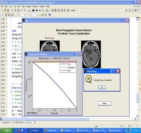
Figure.4 Result of training graph of neural network

Figure.5 Result of normal image classification

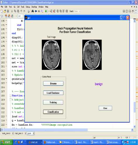
Figure.7 Result of benign image classification

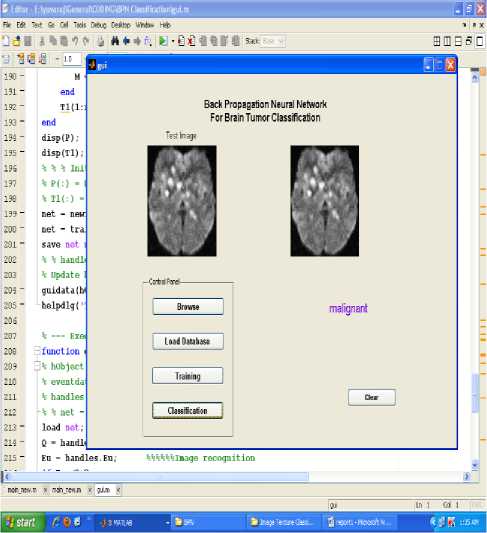
Figure.6 Result of malignant image classification

The most widely used Neural-network learning method is the Back Propagation algorithm. Learning in a neural network involves modifying the weights and biases of the network in order to minimize a cost function. The cost function always includes an error term a measure of how close the network's predictions are to the class labels for the examples in the training set. The activation function considered for each node in the network is the binary sigmoidal function defined (with s = 1) as output = 1/ (1+e-x), where x is the sum of the weighted inputs to that particular node. This is a common function used in many BPN. This function limits the output of all nodes in the network to be between 0 and 1. Note all neural networks are basically trained until the error for each training iteration stopped decreasing.

All classification result could have an error rate and on occasion will either fail to identify an abnormality, or identify an abnormality which is not present. It is common to describe this error rate by the terms true and false positive and true and false negative [11, 12, 13].The performance of the network is derived from the MSE value. No further improvement in the MSE is observed as shown in figure 4 of training graph of the neural network.

• V.    CONCLUSIONS

In this paper an automatic method for classification of brain tumors in to malignant or benign are proposed. Features extracted using principal component analysis was used for training and testing. Back propagation algorithm was used for training, testing and classification of the tumor. BPN is adopted for it has fast speed on training and simple structure Results show that the features extracted can give satisfactory result in analysis and classification of brain tumors.

Experimental result indicates that BPN classifier is workable with an accuracy ranged from 100% to 73%. Further work is to check the performance of the system by increasing the database.