Brain tumor classification using deep convolutional neural networks

The identification of brain tumors represents a vital task with direct implications for diagnosing and treating tumor-related conditions within this organ. Leveraging contemporary research methodologies, especially deep convolutional neural networks (CNNs), holds tremendous potential for enhancing both the precision and efficiency in detecting brain tumors across medical imaging modalities like magnetic resonance imaging (MRI) and computed tomography (CT).

Classification problems are usually solved using traditional machine learning algorithms, but recently deep learning models have become increasingly used. Artificial neural networks, as the flagship among their contemporaries, are capable of identifying patterns and connections hidden from the human eye. While simple fully connected neural networks cope well with classification and regression problems on tabular data, convolutional networks allow solving problems where computer images serve as data [1].

Convolutional neural networks (CNNs) have emerged as a pivotal asset in image processing and pattern recognition, primarily attributed to their capability to discern features from data across various levels of abstraction [2]. Within the realm of brain tumor detection [3], these networks exhibit promise in streamlining and enhancing the image analysis procedure, thereby potentially augmenting the effectiveness of diagnosis and the timely identification of tumor abnormalities [4].

In the context of brain tumor detection, research has previously been conducted using classical machine learn- ing methods [5], however, these have been limited in accuracy and ability to process the complex patterns found in medical images. These approaches often had limited capabilities compared to deep convolutional neural networks (CNNs), which are capable of extracting and analyzing more complex features and patterns from images, improving the accuracy of tumor detection. However, it should be noted that classical machine learning is capable of diagnosing rare diseases more than widespread ones [6, 7].

A range of medical imaging techniques, including radiography, computed tomography (CT), magnetic resonance imaging (MRI), biopsies, and others, are employed to detect diseases, such as brain tumors [8]. These modalities furnish a comprehensive and intricate depiction of the body's internal structures, necessitating meticulous scrutiny to pinpoint pathologies, including tumor growths. Leveraging contemporary deep learning methodologies rooted in convolutional neural networks presents novel opportunities to automate the detection and precise diagnosis [9] of such diseases using medical imaging data.

This research aims to explore the operational principles of deep convolutional neural networks concerning the detection of brain tumors. It will delve into their benefits and obstacles, alongside current research and developmental prospects in this domain. Such an investigation is poised to foster a deeper comprehension of the importance and possibilities associated with the application of these technologies in medical diagnostics.

The aim and objectives of the study

The objective of this study is to conduct a comparative analysis of different convolutional neural networks in their effectiveness for detecting brain tumors in medical MRI images. To accomplish this objective, the following tasks have been outlined:

• 1 .Training various convolutional neural networks: It was necessary to train several variants of models, including a convolutional neural network with its own architecture, as well as models based on Transfer Learning using pre-trained neural networks: Xception, VGG-19 and ResNet-50.

• 2 .Evaluate classification accuracy: Evaluate the accuracy and classification results of each model on the test data set using performance evaluation metrics such as accuracy, recall, F1-measure and error matrix.

• 3 .Comparative analysis of results: Compare the classification results of various models and determine the most effective in terms of detecting brain tumors.

• 4 .Identifying the advantages and limitations of each model: Identify the advantages and disadvantages of each model based on their efficiency, training time, computational resource requirements, and potential applicability in clinical practice.

1.    Literature review

Detection of tumors using traditional methods is timeconsuming and does not allow diagnosing a large volume of data [10], so automatic diagnosis of tumors, supported by image processing and machine learning methods, is an integral part of modern technologies in artificial intelligence systems. A number of studies on this topic have made undeniable advances in machine learning diagnostics, which is encouraging, but challenges remain, such as accurate tumor segmentation and classification.

• S.    Kumar et al. conducted a review involving two-step approaches on 20 scientific papers published between 2000 and 2020 to learn more about tumor detection in MRI images [10]. Following the analysis, the authors determined that CNN methods exhibit superior accuracy with a reduced error rate. This approach enhances image segmentation and spatial localization levels, thereby enhancing performance in comparison to alternative systems.

2.    Materials and methods

The study authored by Refaat, Fatma, Gouda, M., and Omar, Mohamed [11] delves into diagnosing three categories of brain tumors, namely meningiomas, gliomas, and pituitary tumors. The article proposes machine learning algorithms, namely KNN, SVM, and GRNN, aiming to enhance accuracy and diminish diagnostic duration by leveraging publicly available datasets, image-extracted features, data pre-processing techniques, and Principal Component Analysis (PCA). The diagnostic accuracy achieved by the algorithms for tumor diagnosis stands at 97% for KNN, 96.24% for SVM, and 94.7% for GRNN, respectively.

In [12], convolutional neural networks (CNN) were utilized to construct a deep learning system (DLS) for categorizing liver tumors based on enhanced MR images, non-enhanced MR images, and clinical data, including textual and laboratory findings. When using solely unen- hanced images, the CNN exhibited proficient discrimination between malignant and benign liver tumors (AUC 0.946; 95% Acc. 0.914–0.979 vs. 0.951; 0.919–0.982, P=0.664). Integrating unenhanced images with clinical data via a novel CNN notably enhanced performance in distinguishing malignancies such as hepatocellular carcinoma (AUC 0.985; 95% CI 0.960 – 1.000), metastatic tumors (0.998, 0.989 – 1.000), and other primary malignancies (0.963; 0.896– 1.000). Moreover, the agreement with pathology was 91.9 %. Trained on data from various acquisition conditions, DLS amalgamating these models could serve as an accurate and time-efficient auxiliary tool for diagnosing liver tumors in clinical environments.

The study [13] aims to classify and segment brain tumors based on MRI images using machine learning methods. Preprocessing methods, skeletal segmentation and classification using deep convolutional neural networks (CNN) and feature extraction based methods (SVM with combined HOG and LBP features) are used. The study shows classification accuracy: CNN – 98%, SVM – 97%. It should be noted that such accuracy is due to the solution of the binary classification problem and a balanced dataset.

The paper [14] focuses on building a convolutional neural network (CNN)-based brain tumor diagnostic system using the EfficientNetv2s architecture optimized with Ranger and extensive preprocessing. The authors use Transfer Learning to solve the classification problem. The main drawback of the authors of the study is that Ef-ficientNetv2s uses significant computing resources for training and prediction, since it has a large number of different convolutional layers.

The purpose of this review [15] is to provide comprehensive literature on the detection of brain tumors using magnetic resonance imaging to assist researchers. This study encompassed various aspects of brain tumor analysis, including brain tumor anatomy, publicly accessible datasets, techniques for enhancement, segmentation, feature extraction, classification, and the utilization of deep learning, transfer learning, and quantum machine learning methods.

In paper [16], Al-Ayyoub, Mahmoud, Husari, Ghaith, Darwish, Omar, and Alabed, Ahmad introduce a machine learning methodology aimed at discerning the presence of tumors in MRI brain images. Results from experiments indicate that following MRI image preprocessing, the neural network classification algorithm demonstrated superior performance.

The best method for detecting brain tumors is magnetic resonance imaging (MRI). The scanning process generates a huge amount of image data. These images are examined by a radiologist. Manual examination may be prone to error due to the level of complexity of brain tumors and their properties [17].

The dataset was taken from the kaggle.com portal from the Brain Tumor Classification (MRI) open competition. The dataset consists of selected sections of MRI images and contains 7023 jpeg files. The data was distributed into 4 classes: glioma tumor, meningioma tumor, no_tumor (healthy), pituitary tumor. The ratio of the number of files for each class was as follows (Table 1).

Tab. 1. MRI slices distribution for training and testing purposes

Brain Tumor Type	Training	Testing
Glioma	1321	300
Meningioma	1339	306
No tumor	1595	405
Pituitary	1457	300
Total	5712	1311

This is further demonstrated in Fig.1.

3.    Research methodology

In the problem of pattern recognition, the use of convolutional neural networks is widespread. Moreover, today Transfer Learning technology has begun to be actively used [18], which makes it possible to use models pretrained on large data sets to solve various recognition problems from other industries [19].

In order to achieve maximum accuracy in recognizing a brain tumor, it was decided to build our own convolutional neural network model, as well as a Transfer Learning model based on the ResNet50, VGG-16, and Xcep-tion models [20]. This choice of models is due to the fact that each of them uses different approaches to processing graphic information supplied in the form of an array of image pixels. Before describing the structure and features of each of the models, it is necessary to determine the sequence of actions that were performed in the process of comparative analysis of these models. This sequence is shown in Fig. 3.

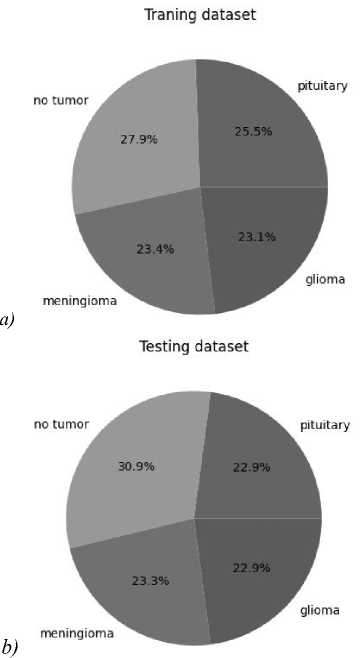
Fig. 1. Pie chart of classes for samples. (а) Training, (b) test

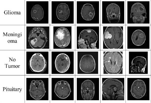
Fig. 2. Dataset classes names: glioma, meningioma, no tumor (healthy), pituitary

Depthwise Separable Convolution is a convolutional neural network technique that splits the convolution operation into two stages: Depthwise Convolution and Pointwise Convolution. This technique can significantly reduce the number of parameters and computational complexity of the model, while maintaining or even increasing its performance.

The operating principle of separable convolution can be divided into two main stages.

Spatial convolution stage. At this stage, each channel of the input image is processed separately using its own filter (kernel). Each channel has its own convolution kernel. This allows the model to account for spatial dependencies in the data.

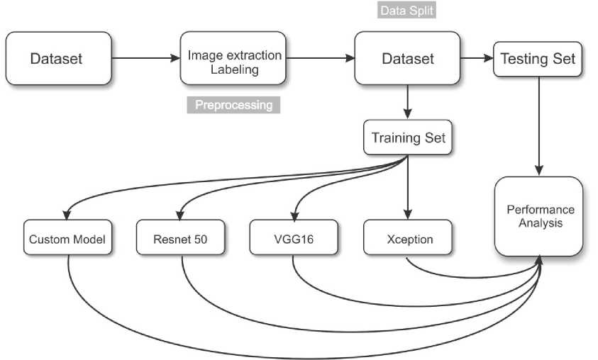
Fig. 3. Model training methodology

After spatial convolution, convolution with a 1×1 kernel (dot convolution) is applied. This operation combines the spatial convolution results for all channels of the input image into a single output image. Thus, spatial information is reduced to one point. The working principle of split convolution is illustrated below (Fig. 4).

Fig. 4. The example of separable convolution

Separable convolution is effectively used in various fields, including medicine, due to the following advantages:

- shared convolution requires less computational resources and memory compared to traditional convolution layers. This is especially important in resource-constrained applications, such as medical applications, where access to large computing power may be limited.

- spatial convolution allows the model to take into account spatial dependencies between pixels in the image. This is especially important in medical problems where structures are important for correct diagnosis and classification.

- separable convolution can help reduce the number of parameters in the model, which can help combat overfitting, especially in the case of small data sets.

- with proper configuration and training, separable convolution can achieve high levels of classification and segmentation accuracy, which is especially important for medical applications where accuracy plays a critical role.

In medicine, separable convolution can be effectively used, for example, for image classification of medical images, segmentation of structures in brain images, analysis of X-ray and tomography images, and many other tasks where high accuracy and efficient use of resources are important.

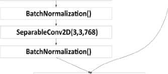
First, we will describe our own convolutional neural network model (Fig. 5). The model consisted of a 224×224 input layer, 3 3×3 convolution layers and 32 filters using ZeroPadding, 4 3×3 convolution layers and 64 filters, batch normalization layers, and a 2×2 Pooling layer. The model also applied separable convolution layers, which were completed with a transformation layer into a Flatten vector. The final dense layer was activated by the Softmax function and gave the probabilities of the image belonging to the class (Glioma, Meningioma, No tumor, Pituitary).

Input (224,224,1)

2eroPadding2D(2,2) I

Conv2D(3,3,S4)

BatchNormalization I

MaxPooling2D(2,2)

Conv2D(3,3,256)                    Conv2D(3,3,64)

I                                             I

BatchNormalization ()                 BatchNormalization!)

Conv2D(3,3,128)                    Conv2D(3,3,128)

В atch No rma li zation ()                 BatchNormalization!)

Z^Z              1

DropOut (0.5)

Dense(256)

DropOut (0.5)

J

Dense(128)

Dense(64)

Dense(32)

Dense{4)

M ax Pool i ng2D (2,2)                   Average Pool i ng2D( 2,2)

SeparableConv2D{3,3,128)           SeparableConv2D(3,3,l)

BatchNormalization!)                BatchNormalization!)

MaxPooling2D(2,2)

SeparableConv2D{3,3,512)

Global MaxPooling2D() I

Dense(1024)

Fig. 5. Structure of own model

Next, a model based on ResNet50 was assembled. The difference between ResNet50 and the previous model was mainly that this model uses residual learning. It avoids retraining the model at various stages and solves the vanishing gradient problem. Specifically for this work, the problem of a vanishing gradient was not identified, however, there were risks that the model could incorrectly determine that an image belongs to a certain class if the objects in the image were similar to each other. ResNet50 layers were used by default with a top classification cutoff of 1000 neurons for the Imagenet database. The structure of the model based on ResNet50 is shown in the figure below (Fig. 6).

Input (224,224,1)

Resnet50Model

Flatten

BatchNormalization

Dence{256)

DropOut{0.5)

BatchNormalization!)

Dense(128)

DropOut(0.5)

BatchNormalization()

Dense(64)

—J— Drop0ut(0.5)

BatchNormalization()

Dense(32)

DropOut(0.5)

BatchNormalizationf)

□ense(4)

Fig. 6. Model structure based on ResNet50

The VGG-16 model is based on classical convolutional layers without using any approaches that improve the recognition process. However, this model has good accuracy due to careful selection of the number of convolution filters and their sizes. The main feature of VGG-16 is the use of traditional convolution methods to avoid computational complexity during training. The structure of the VGG-16-based model is shown in the figure below (Fig. 7).

Before describing the structure of the Xception-based model, we should note its key features and differences from other models. It is known that any convolutional layer processes both information within each channel (spatial) and information between channels simultaneously. The Xception architecture assumes that both of these forms of information can be efficiently processed sequentially, and so it splits conventional convolution into two parts: pointwise convolution

(working only on cross-channel connections) and spatial convolution (working only on spatial connections within channels). By applying this approach, the weight of the trained Xception model is significantly less than the weights of other models. The structure of the Xception-based model is shown in the figure below (Fig. 8).

Input (224,224,1)

VGG16Model

Flatten

BatchNormalization

Dense(2S6)

DropOut{0.5)

BatchNormalization!)

Dense(128)

DropOut(0.5)

BatchNormalization!)

Dense(64)

DropOut(0.5)

BatchNormalization!)

Dense(32)

DropOut(0.5)

BatchNormalization!)

Dense(4)

Fig. 7. Model structure based on VGG-16

4.    Results and discussion

The training was carried out on a computer with the following characteristics:

CPU: Intel core i5 13400;

GPU: NVIDIA RTX 4080, 9728 CUDA cores, 20Gb GDDR6.

The proprietary model demonstrated the highest accuracy and best metrics compared to models using Transfer Learning based on ResNet50, VGG-16 and Xception. This indicates the effectiveness of the developed network architecture for this classification task.

After training and testing all four models, key metrics were analyzed: accuracy, precision, recall, F1-Score, ROC AUC Score for each class and the average value for all classes for the same characteristic.

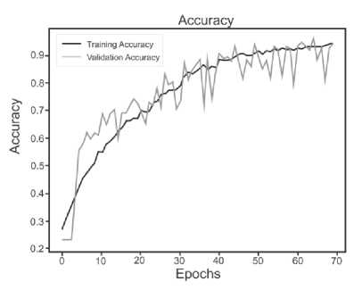
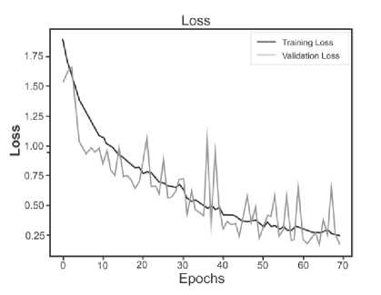
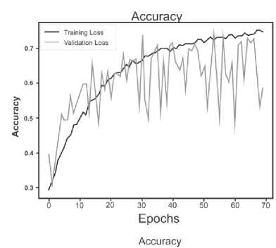
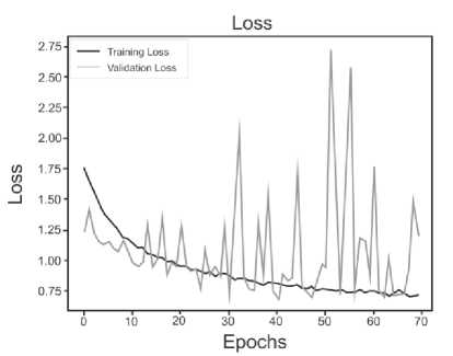
Below are the training histories for each model in the form of Accuracy and Loss graphs (Fig. 9 a – d ).

The best results, as can be seen from the table above, are shown by a model based on its own architecture with selected convolutional layers and an approach based on separable convolution. It is important that for each model the image, when fed to the input of the neural network, was converted to grayscale and then convolution and pooling operations were applied to it. This means that the comparison of models and approaches in this context is correct and technically sound.

Input (224,224,1)

XceptionModel

Flatten

BatchNormalization

Dense(256)

DropOut(0.5)

Batch Norma I ization()

Dense(128)

DropOut(0.5)

BatchNormalization()

Dense(64)

DropOut(O-S)

Batch Normalization^

Dense(32)

DropOut(0.5)

Batch Normalization()

Dense(4)

Fig. 8. Model structure based on Xception

The results of the evaluation metrics are also presented in Table 2.

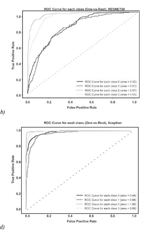
The ROC AUC indicator is also very important when solving classification problems. Visualization of graphs of the ROC AUC Score metric is shown in the figure below (Fig. 10 a – d ).

For each class, the ROC AUC Score of its own model showed a minimum of 100% indicator; with a low degree of error, the model identified only the Meningioma and Pituitary classes due to their external similarity.

It is important to highlight that while Transfer Learning enables the utilization of pre-trained models for addressing analogous issues, in this instance, it did not outperform the performance of the original model architecture. It is possible that for a given data set and classification task, the specific characteristics of the proprietary model were more optimal.

To compare the results, here is table (Table 3), which describes the main results of work on the classification of brain tumors.

The comparison table shows that the potential of Transfer Learning models and a simple convolutional network for solving the problem of classifying medical MRI images is not enough. To bypass the bottleneck, the authors of [22] added an additional one to the main dataset, only after which they were able to improve the accuracy of the model. Regarding the MONAI model, this library contains basic tools for processing medical images and pretrained models capable of recognizing anomalies in them, however, due to the specificity of some tasks and the quality of images, it is not possible to be completely confident in the reliability of the MONAI model.

At first point of view, the VGG-16-based model has a simple architecture, is easy to interpret, and works well on small data sets. However, the tendency to overtrain does not allow using this model fully.

In contrast, the Xception-based model uses deep separable convolution, efficiently learns cross-channel dependencies, and is a lighter model compared to previous architectures. However, it may require more training time than simpler models like VGG-16, and there are some difficulties in interpreting the results.

The model based on the ResNet50 architecture uses residual blocks to combat the problem of gradient decay, high accuracy on various classification tasks. The only thing is that a large number of parameters may require more time and computing resources for training.

Efficient use of parameters, reduced number of calculations, tendency to learn quickly and resistance to overfitting. Such a model requires careful tuning of parameters, which can cause difficulties in interpreting the results. Specifically, in this study, this accuracy rate was achieved by long selection of the number of separable convolutional layers and the number of parameters in each of them.

When choosing a model for practical use in clinical practice, it is important to consider the balance between classification accuracy, training time, computing resource requirements and ease of interpretation of results.

Conclusion

Tab. 2. Results for each model

Model	Metrics (average, weighted average)
	Accuracy	Precision	Recall	F1 Score	ROC AUC Score
Custom CNN	0.93	0.89	0.90	0.85	0.97
Resnet50	0.74	0.61	0.58	0.54	0.88
VGG-16	0.62	0.57	0.52	0.53	0.56
Xception	0.86	0.89	0.90	0.89	0.94

a)

b)

c)

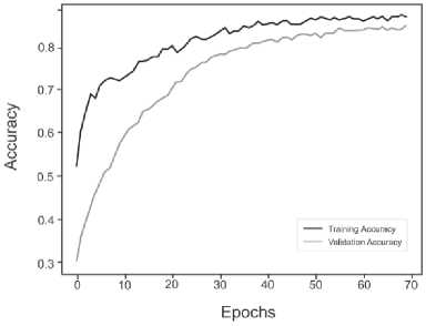
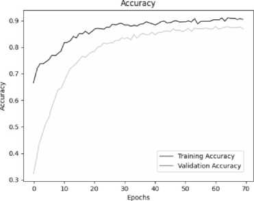
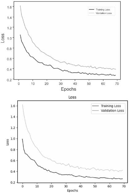
Fig. 9. a) Custom CNN, b) ResNet50, c) VGG-16, d) Xception

a)

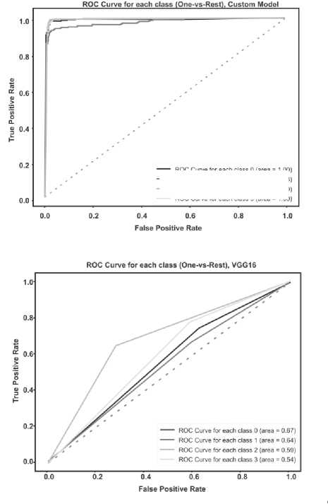
Fig. 10. a) Custom CNN, b) ResNet50, c) VGG-16, d) Xception

---- roc curve tor each class о (area = i .00] — ROC Curve for each class 1 (area = 0.98) ---- ROC Curve for each class 2 (area = 1.00) ROC Curve for each class 3 (area = 1.00)

c)

Tab. 3. Model comparison with related works

	Reference	Accuracy (%)	Classification Method	Classification type	Dataset, reference
1	[21], kaggle notebook kernel	72.8	Simple CNN with 4 layers	Multi	Brain tumor dataset [17]
2	[22], kaggle notebook kernel	91	EfficientNetB0	Multi	Brain tumor dataset [17], private dataset containing 950 images
3	[23], kaggle notebook kernel	86	MONAI framework model	Multi	Brain tumor dataset [17]
4	Developed model	93	CustomCNN	Multi	Brain tumor dataset [17]

Conclusion

The most successful and effective model turned out to be our own model, which includes the use of separable convolution technology, batch normalization and the use of ZeroPadding at some stages of data processing. This architecture demonstrated the highest rates of accuracy and other quality metrics.

It is important to note that the model built on the Xception neural network architecture also showed good results. This indicates the potential and effectiveness of this architecture in solving the problem of classifying brain tumors using MRI data.

The findings from this study suggest that future efforts should include parameter optimization and further experimentation to enhance the accuracy of brain tumor classification using MRI data. These results underscore the significance of employing deep learning techniques in the medical domain to automate diagnosis and enhance disease detection precision.