Buckling of orthotropic plates with the two free edges loaded for the pure in-plane bending moment

The buckling problem of rectangular plates involving two opposite edges loaded with distributed stress has been studied for a long time. Bubnov [1] and Timoshenko [2] were the first who solved this problem for isotropic plates. The same buckling problem of orthotropic plates was solved by Lekhnitskii [3]. These classical solutions in the form of trigonometric series are obtained for plates with simply-supported edges. The Ritz energy method is used to define critical loads because the partial differential equation of stability involving the floating factor makes integration difficult. Reddy [4] and Whitney [5] used the Ritz method for solving this buckling problem of composite plates with simply-supported edges loaded even with compressed stress.

Therefore, the buckling of plates was studied mostly in widespread boundary conditions i.e. simply-supported edges. There is only one reference to Nolke’s paper [6] in Bloom and Coffin’s manual [7], in which the same problem is solved for the plate with two clamped edges.

So we have decided to solve the buckling problem of the orthotropic plate with two free and two simply-supported edges loaded for the pure in-plane bending moment. We have not been solving the buckling problem of orthotropic plate loaded for line-distributed forces due to the limits. The solutions for buckling of orthotropic plate loaded for even compressed forces are given in Leissa’s manual [8].

In our research the solution of an original equation for stability analysis is based on the Levy-type solution procedure. It allows the reduction of partial differential equation to ordinary differential equation. The latter is solved by the finite difference method. Linear homogeneous algebraic combined equations had been used. The determination of the critical load is reduced to the calculation of buckling coefficient corresponding to minimal eigenvalue of combined equations. The solutions for isotropic plate buckling and symmetrically reinforced orthotropic plate had been obtained as well.

The buckling solution. We have considered an orthotropic plate the middle plane of which is corresponds to the Cartesian coordinates xy . The dimensions of the plate are a and b as showninthefigurebelow. Edgesalongthe y =0and y = b are free, and edges loaded with the line-distributed stress along the x = 0 and x = a are simply-supported. The load distribution corresponds to two bending in-plane moments.

The equation for the stability analysis of orthotropic plate is given as follows

D^^ + 2 ( D 2 + 2 D 33) , , + D 22

¹¹ d x^{4 v 12       33} )dx ² d y ^{2     22}

d ⁴ w dy⁴

2  22

- N ^ r — 2 N L ^- w — N ; “ T = 0, x d x ²       xy d x d y      y 8y y

where w = w ( x,y ) is the transverse displacement, D ₁₁, D ₁₂, D ₂₂, D ₃₃ are the bending stiffnesses of the plate given in [9]. №_x, N y , N x_y are membrane stresses corresponding to the subcritical state of the plate.

We assume that the origin stressed state corresponds to it’s pure in-plane bend. Then membrane subcritical stresses could be define as

N ; =— N fl — 2 y 1, N L = 0, N ^ = 0,        (2)

x                              xy             y

I b)

where N isthemaximalstressvalueatedges y =0, y = b .

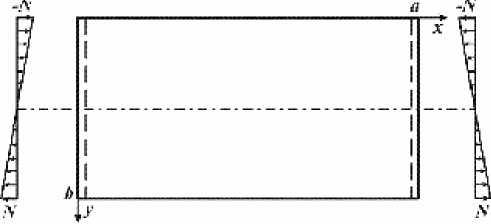
Plate stress

Equation (1) with (2) taken in account is depicted as 44

D11 — + 2( D + 2 D33) -—2- + dx               dx dy d w   f    y W w

+ D     + N 1 - 2       = 0.          (3)

²² dy ⁴      I      b J d xx

Let us consider the boundary conditions. Displacements and bending moments are equal to null when the edges are simply-supported (x =0 x = a). Generalized forces and bending moments are equal to null when the edges are free (y = 0 y = b) [9]. These boundary conditions could be derived from plate displacement w can be presented as w = 0, D d— + D d— = 0 atx = 0andx = a,(4)

and           ⁵ x ’

D„ ^ ^ w + D „ ^ 2 ^ = 0

12 dx2      22 dy2

Dn    + ( D 2 + 4 D 3 3) —= 0

22              1233

dydx aty =0andy=b.(5)

Thereby, the buckling problem of plate is reduced to the definition of parameter N corresponding to nonzero solution of the boundary-value problem (3, 4) and (5).

The fact that there are edges simply supported makes the representation of solution possible (3) in Levy-type form

w ⁽ x , У ) = £ W m ⁽ У ^)si n ¹ m X .            (6)

m = 1

Here m is the amount of half-waves along side a , w_m ( y ) is an unknown function, 1 m = m п/ a . However, there no necessity to approximate the solution with series (6) in the problem we overlook. It’s enough to keep one term of the series corresponding to m = 1. Indeed, the buckling of the plate doesn’t experience resistance along side a . Therefore, the plate’s bend takes place with formation of only one halfwave along side a . This half-wave has a maximal amplitude attheedge y =0, whichdecreasealong y totheedge y = b .

Now the solution of the equation (3) can be presented as

w ( x , y ) = w ( y ) sin 1 x .             (7)

Here w ( y ) = w 1 ( y ), l = п/ a .

Substituting of (7) into equation (3) gives the ordinary differential equation

DU1w - 2(D12 + 2D33)—— + dy2

+ D22 d4w - N Г - 2 yw = 0.(8)

1 2 dy ⁴ I b J

Here w = w ( y ).

Substituting of (7) into boundary conditions (5) gives

D2I2 w - D 22 dw = 0,(9)

dy ²

-D22 dw + (D12 + 4D33)12 dw = 0,(10)

dy3

where y =0, y = b .

The difference method is used to solve equation (8). Let’s divide side b into numerous equal parts. The points of division have the following coordinates

У,= 5(i -1),      i = 1,2,..., k .(11)

Here s = b / n and is subinterval, k = n+ 1.

The approximation of derivatives corresponding arbitrary point y gives dw)    1 /x

— = —( - w 1 + w ,₊1)

1                               i -1          i +1 V , dy ),2

Г d w) 1 /.

I I = —⁽ w i - 1 ^{- 2 w}, ^{+ w}, + 1 ),

( dy ),

I d3 w I 1 z„

I 7т I = , Jw-2 + 2 wi-1 - 2w+1 + w,+2), dy3

d4 w) 1 / л с лл

7? I = — (wi-2 - 4wi-1 + 6wi - 4wi+1 + wi+2) . dy4

Here w , = w ( y , ).

Substituting of (12) into (8) gives the following finite difference approximation of equation (8):

D Д² w, - 2 D ^{12 + 2} D ³³ A + D; B - N ^f 1 - 2 ^{У 1} w, = 0 .(13)

^{11 i} 5²               1 2 5⁴ *       ( b J ⁱ

Here A_i and B_i are defined as

A , = w - 1 - 2 w , + w _M,

B = w . - 4 w ,+ 6 w - 4 w ^,+ w₂.      (14)

i         i - 2            i - 1            i           i + 1         i + 2                  ' '

The transformation of equation (8) into dimensionless form gives

22n ап w, - 2p n a, +2 B, - Пt, w, = 0 , ап where ti = 1 – 2(i–1)/n, а = DU bL R= D12 + 2 D33

D ₂₂ a          D ₁₁ D ₂₂

Nb ² n = I .

^D 11 ^D 22

Here n is a non dimensional buckling coefficient.

Equation (15) writing for all points ( i =1,2,…, k ) represents linear algebraic combined equations, however, including outside edge points. The substituting of i =1 and i = k to equalities (14) gives

A , = w ₀ - 2 w 1 + w₂ ,

B , = w _ 1 - 4 w ₀ + 6 w 1 - 4 w ₂ + w₃         (18)

and

A k = w k - 1 - ^{2 w}k ⁺ w k + 1 ,

^Bk = w k - 2 - ⁴ w k - 1 ^{+ 6} w k - ⁴ w k + 1 ⁺ w k + 2 .         ⁽¹⁹⁾

Therefore, w _–1, w ₀, w_{k +1}, w_{k +2} are outside edge points. It should be noted that unknown w ₀ and w_{k +1} are also including in B ₂ B_{k –1}, giving

B 2 = w ₀ - 4 w 1 + 6 w ₂ - 4 w ₃ + w ₄,

^Bk - 1 = w k - 3 - ⁴ w k - 2 ^{+ 6} w k - 1 - ⁴ w k ⁺ w k + 1 .        ⁽²⁰⁾

Four equations need to define four outside edge unknowns. These equations can be obtained by finite-difference approximation of boundary conditions (9, 10). By substituting of (12) into (9), and of (10) with i =1 i = k ,we obtain

n

Р 1 п w 1-- ( w ₀ -2 w 1 + w ₂) = 0,

а

Р1п wk--(wk-1 -2wk + wk+1) = 0,(21)

а where e1         / .

D ₁₁ D ₂₂

Equations (21) give

w0 = (r1 + 2)w1 - w2, wk+1 = (r + 2)wk - wk-1, where r 1 = аР1п2/n2.

Substituting of (12) into (10) with i =1and i = k gives

--(-w-1 + 2w0 - 2w2 + w3) + (P1 + 402 )п2 (-w0 + w2) = 0,(24) а n2

⁽ - w k - 2 + ^{2 w}k - 1 - ^{2 w}k + 1 ^{+ w}k + 2 ) ⁺

а

+(P1 + 4Р2)п2(-wk-1 + wk+1) = 0, where

₽ 2 =

^D 33

^D 11 ^D 22

Equations (24) in accordance with (23) give w-1 = (2 + r + 4r2)(r1 + 2) w1 - 2(2 + r1 + 4r2) w2 + w3, (26)

w k + 2 = w k - 2 - ^{2(2 +} r ^{+ 4} r 2 ) w k - 1 ^{+ (2 +} r ^{+ 4} r 2 ⁾⁽ r ^{+ 2)} w k , where r ₂ = аР₂п²/ n ².

So, equalities (23) and (26) define four outside edge unknowns. Substituting of (23) and (26) into (18, 19) and (20) gives

A 1 = r l w 1 , A k = r l w k                ⁽²⁷⁾

and

B l = gw - 2 fwi + 2 W 3 ,

B ₂ = vw 1 + 5 w ₂ - 4 w ₃ + w ₄,            (28)

^B k -1 = ^W k -3 ^{- 4 W} k -2 ^{+ 5 W} k -1 ^{+ VW} k ,

B k = ^{2 W} k -2 ^{- 2} f ^W k -1 ⁺ g ^W k -

Here g =6– 4 u + uf , f =2+ r ₁+ 4 r ₂, u = r ₁ +2,n= r ₂–2.It should be noted that A_i ( i =2,…, k – 1) and B_i ( i =3,…, k – 2) are still defined by equations (14).

Thereby, homogeneous algebraic linear combined equations n4

an2wi - 2Pn2Ai +---Bi -nti wi = 0 , an

( i =1,2,…, k )                    (29)

the approximated differential equation (8) contains unknown
w 1, w	2, ..., wk only.
Combined equation (29) could be presented as the
following matrix equation
		( D -n T)W = 0,             (30)
where
	D =	4 an2 E - 2Р n 2 A + —в B .         (31)
		an
Here
	w , 1        Г t 1    0 Л 01
	w„          0 t, Л 0
	W = ^
	M      л л л л
	w k        [ 0  0 Л tk
	1 r 1	M
	1 -2   1	M
	1 -2	1M
	1	-2 1 M
A = ^	Л Л Л	Л Л -M Л Л Л Л Л	,
		M 1 -2  1
		M      1 -2 1
		M           1  -2 1
		M                    r 1

So, the problem we have considered has been reduced to an eigenvalue problem (30). Minimal eigenvalue of linear combined equations determine the value of the non dimensional buckling coefficient h _cr . The accuracy of calculations is estimated by the comparison of results obtaining different values k . Critical stress N_cr is defined by the following equation

DD

N c =П                      (32)

The value of n_cr depends on parameters a, P 1 , P₂ which contain all the information about the size of the plate and its bending stiffnesses.

Examples . The first example we overlook is that of an isotropic plate. Bending stiffnesses at this case are defined by the following expressions.

h ³

D ii = D 22 = ^E 12,

D₁₂ =vEh- , D₃₃ = 1-^ E — ,     (33)

12        12, 33      2     12, where h - is the thickness of plate, E =E/(1 - ц2). Here £ is the modulus of elasticity, m is Poisson’s coefficient.

Expressions (16), (22) and (25) give us a = 1/ c2, P = 1,

P l =ц, P 2 = (1 -ц)/2.

Here c = a/b is the ratio of the plate’s sides. In fact, the buckling coefficient depends on parameter c only. Dependence of n_cr on c has been studied for m = 0,3, n = 50. Parameter c has varied within 1…5. The data is shown in table 1.

The buckling coefficient could also be represented by an expression obtained by the least-squares method, from which we get

18.9695

^{П сг} = ( с - 0.272бГ⁵ 9 .

In the second example we have overlooked the plate formed from unidirectional or orthogonal reinforced layers which reinforce axes form angles ± ф with axis x .

If there is a large amount of layers, the plate’s structure could be considered as homogeneous and orthotropic. Then the bending stiffnesses are defined as

Г g -2 f 2 M 1 V 5 -4 1 M 1 -4 6 -4 1 M 1 -4 6 -4 1 M «Л Л Л Л Л Л -M Л Л Л Л Л л1 M 1 -4 6 -4 1 M 1 -4 6 -4 1 M 1 -4 5 V M 2 -2 f g where

h ³                h ³

11      11 12 , 22       ²²12 ,

D 12 = A 12^ , D 33 = A 33 12,           (35)

A 11 = ^E 1 ^C ф ^{+ E} 2 ⁵ ф ^{+ 2 E} 12 ^C ф ⁵ ф , A 12 = ^E 1 ^Ц12 ^{+ ( E} 1 ^{+ E} 2 - ^{2 E} 12 ) ^C ф ⁵ ф ,

A 22 = E 1 5 ф ⁴ + E 2 с ф ⁴ + 2 E 12 C ф ² 5 ф ²

^A 33

= ^{( E} 1 ^{+ E} 2 -

,

^{2 E} 1^Ц12 ) ^C ф ⁵ ф ⁺ G 12 ^{( C} ф

-

The unspecified array of the matrix’s cells A and B are equal to null. E is the identity matrix.

E 12 = E 1 Ц 12 + 2 G 12 , ^E 1= ,   ,E¹,, , ^E 2 =

^{1    Ц}12^Ц21

C ф = cos ф, 5 ф = sin ф .

5 ф ²)², E 2

^{1   Ц}12^Ц21

Here E ₁, E ₂ are modulus of elasticity along the reinforcedirection and along the transverse direction respectively, G 12 is the rigidity modulus, ц₁₂, ц₂₁ are Poison’s coefficients.

The substituting of (35) into (16), (22) and (25) gives

1 Aik R - A 12 + ² A 33

= c4A 22^{, e} = _x A A ,

P 1 = , ^A 12       P₂ = , ^{A 33}

A ₁₁ A ₂₂            A ₁₁ A ₂₂

Thereby, the buckling coefficient depends on the

parameter c and the angle ф for the orthotropic plate. A

transformation of the expression Nb ²

Her = I cr     D11D22

to

'b

^N cr ^{b 2}

D 1

makes the param etrical analysis more convenient. Here П сг = H er V К 1 f 22 , f 1 = A 11 / E , f 22 = A 2 / E ,

D = E\ — ¹¹ 12

.

We have finished studying the dependence of n_cr on c and ф. The calculation has been done for carbon-filled plastic with elastic characteristics E ₁ = 142.8 GPa , E ₂ = 9.13 GPa , G ₁₂ = 5.49 GPa , E 1 = 142.8 GPa , ц₁₂ = 0.02, ц₂₁ = 0.32. The data is shown in table 2.

The maximal buckling coefficient for the square plate realizes with angle ф = 14E. The optimal angle tends to 22E with an elongation increase.

The buckling problem of orthotropic plates with two free unloaded edges and two simply-supported edges loaded for in-plane line-distributed stress had been solved. The definition of the critical load has been reduced to the calculation of a non dimensional buckling coefficient. The

value of the coefficient depends on plate’s geometric and elastic parameters. The finite difference method had been used to solve the aforementioned problem. The buckling coefficient had been defined as a minimal eigenvalue of homogeneous linear combined equations approximating the boundary-value problem; it has been solved for the isotropic plate and the orthotropic symmetrically reinforced plate. Different elongation angles of optimal reinforcement for the plates had been defined. We have completed studying the influence of the side ratio and reinforcement angles on wave generation.