Buffering Strategies in Optical Packet Switching

Published Online March 2016 in MECS DOI: 10.5815/ijcnis.2016.03.03

• III.    Buffering Schemes

Packet switching is a network communications method that groups all transmitted data into suitably-sized blocks, called packets. The data packets are of fixed size and some header bytes are added before transmission. Header contains information such as destination address, sender address, size of payload etc. The data packets of message are transmitted by one node to another till it reaches its destination. As the header has to be processed at each switch node, it is desirable that header has a relatively low fixed bit rates. The use of fixed length packets can significantly simplify the packet contention resolution and buffering, packet routing as well as packet synchronization. The packet switching does not require a link with a dedicated and reserved bandwidth. Depending on the network and on the available bandwidth on different line any packet may take several possible routes to reach the destination. In such a case, a sequence number is included in the packets to ensure that the packets will not be misinterpreted if they arrive out of order.

Contention among the packets arises when two or more than two packets try to occupy same outgoing fiber. Buffering is a phenomenon, by which contending packets are stored in fiber delay lines. Various fiber delay lines designs are possible where contending packets are placed [5-13]. These designs are well known as optical switches. In these switches buffering can be done at the input, output or within the switch. Input buffering scheme leads to the head on blocking, thus not preferred [14-15]. In OPS two most preferred buffering schemes are output and shared buffering schemes.

In general optical fiber delay lines based buffers can be classified into two categories: travelling-type and recirculating type.

• •    A travelling–type buffer generally consist of multiple optical fiber delay–lines whose lengths are equivalent to multiples of a packet duration T , and optical switches to select delay lines.

• •    The re-circulating type buffer is more flexible than the travelling type buffer because the storage time of packet can be adjusted by changing the number of revolutions of the data in the buffer. In principle recirculating type buffer acts like random access memory where storage time depends on the number of circulations.

• A.    Output Buffering

In output buffering scheme (Fig. 1), a separate buffer is placed at the each output port of the switch and arriving packets are transferred to appropriate output port and will be processed such that FIFO can be maintained. In the output queuing structure no internal blocking occurs. Therefore large throughput is achievable [7].

Output Buffering Scheme

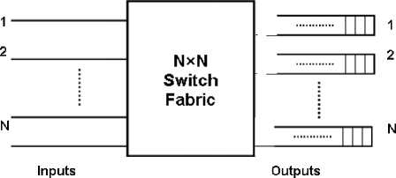
Fig.1. Schematic of Output Buffering Scheme

Output buffering gives the best achievable waiting time performance compared to any other queuing approach. However, for this approach also the large buffer size requirement is a matter of concern, because the larger the required buffer size, the larger would be the cost.

Shared Buffering Scheme

м

N

Inputs

(N+M)x(N+M) Switch Fabric

N

Outputs

Fig.2. Schematic of Shared Buffering Scheme

• B.    Shared Buffering

The above discussed output buffering schemes are not cost efficient because at each port separate buffer is required. Therefore hardware complexity is very large. In the shared buffering scheme (Fig. 2) packets for all the outputs are stored in the common shared buffer. Therefore hardware complexity is less and still higher throughput is achievable.

Here, in effect, a separate queue is formed for each output of the switch, but physically, all queued packets in the switch share the same buffer space. Due to this kind of queuing, we get advantages of output buffer queuing i.e., less waiting time and at the same time saving a lot of buffer space. However, packet loss probability of switch using output buffer queuing is a little better than shared buffer queuing, but that is immaterial with respect to the amount of buffer space saved due to the shared buffer technique.

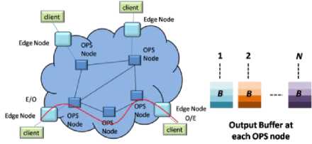
Fig.3. Schematic of OPS Network with Output Buffer at Each Node

In this work we will only consider shared and output buffering of the contending information. Schematic of OPS network with output buffer at each node is shown in Fig. 3. Here, at each node with ‘ N’ input and output links a maximum of ‘ BN’ contending packets and for each output ‘ B’ packets can be stored separately. In figure 4, schematic of OPS network with shared buffer at each node is shown. Here, at each node with ‘ N’ input and output links can store a maximum of ‘ B’ contending packets can be stored in shared manner.

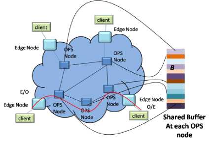
Fig.4. Schematic of OPS Network with Shared Buffer at Each Node

• C.    Load Balancing

Using the above discussion, the optical packet switch will be placed on the nodes R1-R6 and thus buffering will be implemented on these nodes only.

As shown in the figure 5, there are more than one route to reach node D form node C. In networks distance is counted in terms of number of node traversed and known as hops. So from C to D the shortest path is R1-R3-R4. The other two paths R1-R2-R3-R4 and R1-R2-R5-R4 four hops away. As from C to D the shortest path is R1-R3-R4, most of the traffic will follow this path and sooner or later this path will become congested and either packet will be buffered or they will be dropped. To solve congestion some packet my take longer route to reach its destination and thus path R1-R3-R4 is becomes free after sometime, this phenomenon is known as load balancing.

Fig.5. Schematic of OPS Network with Load Balancing Scheme

• IV.    Simulation Methodology

This section presents the simulation methodology. The important network parameters are:

Network Throughput: It refers to the volume of data that can flow through a network, or in other words, the fraction of the generated request which can be served.

Network Load: In networking, load refers to the amount of data (traffic) being carried by the network.

Network Delay: It is an important design and performance characteristic of data network. The delay of a network specifies how long it takes for a request to travel across the network from one node or endpoint to another. Delay may differ slightly, depending on the location of the specific pair of communicating nodes.

• A. Simulation Framework

The simulation is performed in MATLAB. The simulator is a random event generator and well known as Monte Carlo simulation. In the simulation random traffic model is considered. In the simulation we assumed the following

• 1.    Request can be generated at any of the input with probability p .

• 2.    Each request is equally likely to go to any of the output with probability ¹ , where N is the number N

of outputs.

The probability that K requests arrive for a particular output is given by

K         N - K

p[K] = NC I — I | 1 - — I

KIN J I N J

In the simulation synchronous network is considered hence time is divided into slots. Therefore following assumptions are made.

• 1 . The requests can be generated at the slot boundary only.

The simulation steps are shown in figure 6 to 8.

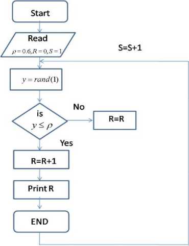
Fig.6. Flow Chart for Request Generation

In fig. 6 flowchart for generation of information is described. The parameters are as defined below:

• •    R= Number of request generated (packets)

• •    p =load

• •    S= Slot for Simulation

• •    Y= Random number

The figure, 6 shows the flow chart for the request generation. Here, for a particular slot a random number ‘ y ’ generated and compared with the considered load (for example 0.6 in figure) if condition is true than a request is generated, otherwise it is considered that no new request is generated. This process is again repeated for the next slot, until the simulation completes.

In figure 7 the flow chart for the destination assignment is shown. Over here is a request is generated then a destination is assigned randomly. In the model uniform random structure is considered.

In flow chart 8, the buffer management process is described. Over here, first buffer is checked and if there is already pending request in the buffer, then it will be served over incoming request. If buffer is free, i.e., no pending request in the buffer, then it will be served. It is noticeable that the buffered request will be given priority over incoming requests. If request cannot be placed in the buffer, the arriving requests are drooped.

• •    R= Number of request generated (packets)

• •    p =load

• •    S= Slot for Simulation

• •    Y= Random number

• •    J= Assigned Destination

• •    L =Loss

• •    B =Size of buffer

• •    C =Counter of packets in the buffer

• •    D =Delay of packets

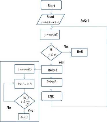
Fig.7. Flow Chart for Request Generation and Server Assignment

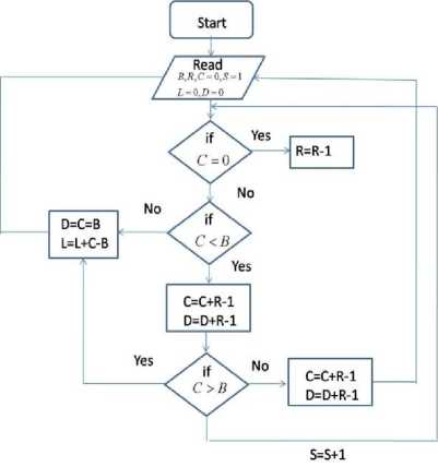
Fig.8. Flow Chart for Buffer Assignment

• V.    Results

In the simulation we have considered a 6 nodes bidirectional network. Here the source node is node 1 while destination node is node 6.

The shortest route is 1-5-4-6-2, with travelled distance as 1.36. In general it is assumed that the distance between the adjacent nodes will be some hundreds of kilometers. Therefore the travelled distance would be 1.36x1000=1360 km.

Assuming data propagation speed in fiber as 2x108 m/s.

Then the propagation time would be (1360x1000)/2x108= 6.8 ms.

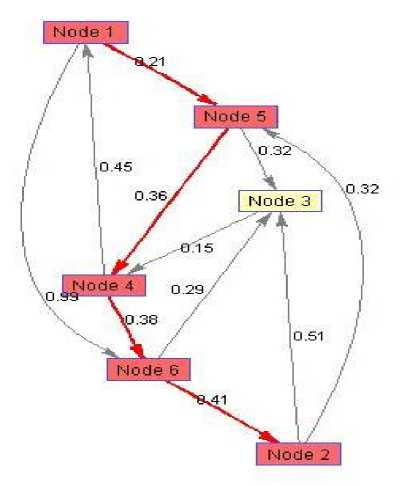
Fig.9. Network under Consideration

Considering that in core network, packet is of size 100000 bits and generation rate is 10Gbps. Then unit slot duration is 100000/1010=10 micro second. Considering the buffering of 16 packets, then the maximum buffering time would be 160 micro second.

Therefore, network propagation time much larger in comparison to buffering time.

Considering, a node in the network with 4 inputs and outputs lines without any buffer. Here, at the load of 0.8, 25 to 30 percent packets lost, depending on the size of the switch or number of input links (Fig.10).

This loss is huge, and to save these packets either deflection routing or buffering can be used. In deflection routing no extra hardware is required, while in case of buffering some mechanism is needed at each node to buffer the contending packets.

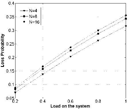
Fig.10. Four Inputs and Outputs Node Without and Buffer

Considering, network in Fig.9, let from node 5 and node 3 two packets arrive for node 4, then one packet will be processed and other will be deflected. Let packet from node 3 is processed then packet from node 5 will be deflected towards the node1 from where it will be either send back to node 4 or will again be deflected towards node 5. Thus looping may occur, packet will reach at the same node where it was generated after traversing a distance of 1020 km. therefore deflection routing is not a good idea in optical networks.

The buffering of contending packets is done in either shared manner or in dedicated buffering scheme. This dedicated buffer can be placed either at the input or at the output of the switch. The input buffering scheme is not preferred due to the head on blocking. Therefore in this work, output and shared buffering scheme is considered.

• A.    Output Buffering:

In Fig. 11-14, simulation results in terms of packet loss probability and average delay for output buffering is discussed.

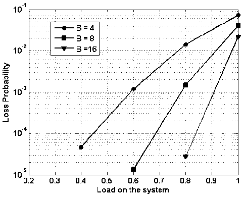
Fig.11. Packet Loss Probability vs. Load on the System with Changing Buffering Capacity

In figure 11, packet loss probability vs. load on the system is presented while assuming 4x4 nodes with buffering capacity of 4, 8 and 16 packets for each node. It is observable that as the load increases the packet loss probability also increases. However, as the buffering capacity increases the packet loss probability decreases. At the moderate load of 0.6, with buffering of 16, 8 and 4 packets, the packet loss probability is approximately, 3 x 10 - 5 , 2 x 10 ^{- 3} and 1.5 x 10 ^{- 2} respectively. Therefore it can be summarized that the buffering capacity has deep impact on the over-all packet loss probability.

In Fig. 12, average delay vs. load on the system is while assuming 4x4 nodes with buffering capacity of 4, 8 and 16 packets for each node. It is obvious from the figure as the load increases the average delay increases. It can also be visualized form the figure that as the buffering capacity increases the average delay also increases. At lower and moderate load (<0.6) average delay is independent of buffering capacity. As load crosses 0.8 mark, thereafter average delay shoots up.

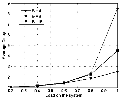
Fig.12. Average Delay vs. Load on the System with Varying Buffering Capacity

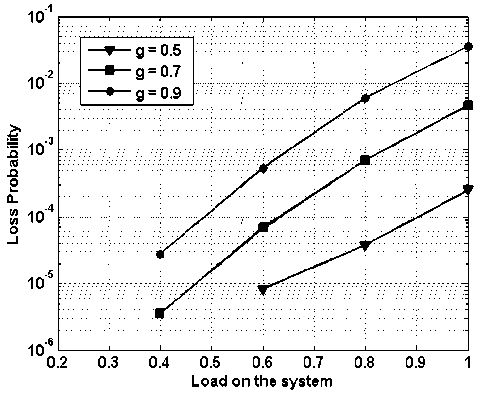
Fig.13. Packet Loss Probability vs. Load on the System with Fix Buffering Capacity of 4, with Load Balancing

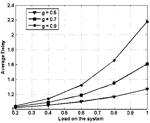
Fig.14. Average Delay vs. Load on the System with Fix Buffering Capacity of 4, with Load Balancing

• B.    Shared Buffering

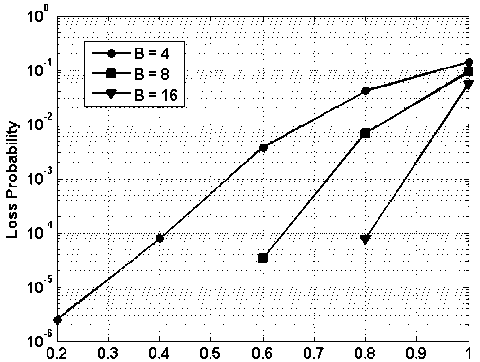
In figure 15-18, results for shared buffering scheme are presented. In figure 15, packet loss probability vs. load on the system is presented while assuming 4x4 node i.e., 4 input and 4 output and buffering of 4, 8 and 16 packets. At the load of 0.8, with buffering capacity of 4, 8 and 16 packets, the packet loss probability is 0 4 x 10 - 2 ,D9 x 10 ^{- 3} and □ 1 x 10 - 4 respectively.

Thus by increasing the buffer space by four fold i.e., from 4 to 16, the packet loss probability is improved by a factor of 400. In case of the output buffering at the load of 0.8, the packet loss rate is 3 x 10 ^{- 5}, however in case of shared buffering the packet loss rate is □ 1 x 10 - 4 . Therefore in case of output buffered system, packet loss better by a factor of three only. But in case of shared buffering the total buffer space is 16, but in case of output queued system is 64. Hence, the performance of the shared buffering is much superior than that of output queued system with much complex controlling algorithm.

In Fig. 13, packet loss probability vs. load on the system is presented while assuming 4x4 node i.e., 4 input and 4 output and buffering of 4 packets. However, load balancing scheme is applied. In the figure ‘ g ’ represents the fraction of traffic routed to global network. For global factor ‘ g =0.5’ the packet loss probability, improves by a factor of 100 in comparison to ‘g=0.9’.

In Fig. 14, average delay vs. load on the system is presented for similar configuration as in figure 13. Comparing with figure 12, the average delay has reduced considerably and this difference is more prominent at the higher loads. For ‘ g =0.5’ the average delay at the load one is reduced by approximate 7 slots. Similarly results for ‘ g =0.9’, where the average delay is recued by 6 slots. It must be remembered that, load balancing scheme reduces loss probability and average delay on local node only, however propagation delay increases as some part of the traffic will follow different path.

Load on the system

Fig.15. Packet Loss Probability vs. Load on the System with Varying Shared Buffering Capacity

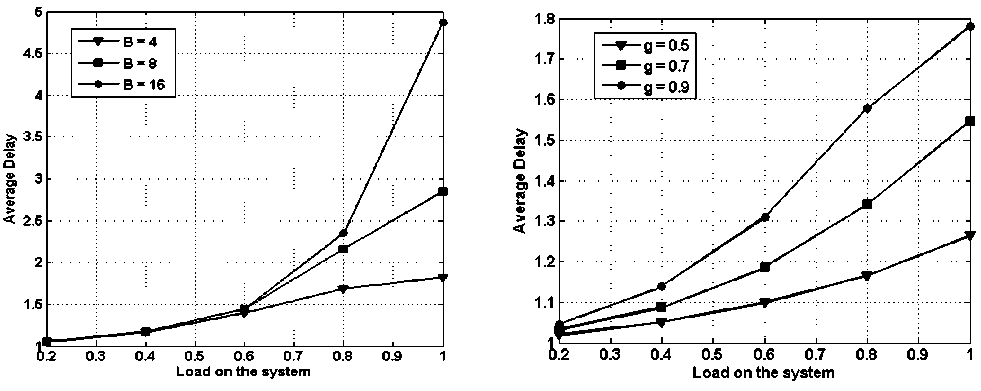
Fig.18. Average Delay vs. Load on the System with Fix Shared Buffering Capacity of 4, with Load Balancing

Fig.16. Average Delay vs. Load on the System with Varying Shared Buffering Capacity

In Fig. 16, average delay vs. load on the system is presented while assuming 4x4 node i.e., 4 input and 4 output and buffering of 4, 8 and 16 packets. The average delay remains nearly same till load reaches 0.6 and in fact average delay is independent of buffering capacity. The average delay is of 5 slots for B =16, which is much less that the output queued system (8.5 slots). Therefore, the average delay performance of the shared buffer is much better than that of output queued system.

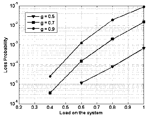
Fig.17. Packet Loss Probability vs. Load on the System with Fix Shared Buffering Capacity of 4, with Load Balancing

In Fig. 17, packet loss probability vs. load on the system is presented while assuming 4x4 node i.e., 4 input and 4 output and buffering of 4 packets in shared manner. In the figure ‘ g ’ represents the fraction of traffic routed to global network. At the load of 0.6, the packet loss performance of the shared and output buffered system is nearly same (Figure 13 and 17). Thus with much reduced buffering requirements shared buffering scheme, along with load balancing scheme provide very effective solution.

In Fig. 18, average delay vs. load on the system is presented while assuming 4x4 node i.e., 4 input and 4 output and shared buffering of 4 packets. However, load balancing scheme is applied. Comparing with figure 16 and 18 the average delay has reduced considerably and this difference is more prominent at the higher loads.

• VI.    Conclusions

In this paper, an important switching problem, contention among the packet is discussed and possible solution: deflection routing and buffering of packets is detailed. For example a six node network is considered with 11 links. Simulation is performed to obtain packet loss rate and average delay and following conclusions can be made:

• 1.    Buffering reduces the packet loss rate.

• 2.    Average delay during buffering is much less then the propagation delay in the network.

• 3.    Load balancing scheme reduces the loss rate at the contending node.

• 4.    Deflection routing is needed when load balancing scheme is to be used to route packets to alternative paths.

• 5.    Load balancing of data traffic reduces traffic at the contending nodes thus both loss rate and average delay reduces.

• 6.    However, due to the load balancing need of deflection routing may enhance as more numbers of packets will follow different paths.

Thus it can be concluded that buffering is an essential and important part in optical packet switching systems.