Building an integral measure of the quality of life of constituent entities of the Russian Federation using the principal component analysis

Автор: Zhgun Tatyana Valentinovna

Журнал: Economic and Social Changes: Facts, Trends, Forecast @volnc-esc-en

Рубрика: Modeling and forecasting of socio-economic processes

Статья в выпуске: 2 (50) т.10, 2017 года.

Бесплатный доступ

Social policy just like any other type of policy is an element of the management system. For effective social policy it is necessary to know the trends and quantitative characteristics of social development dynamics. The purpose for the research is to build an objective composite index to measure and compare the quality of life in constituent entities of the Russian Federation. Such an index is particularly useful in Russia which is undergoing the process of transformations amid increasing social and economic inequality. Objective complex assessment of the quality of life can play a major role in reducing such inequality in Russia. The author implements the algorithm of building a latent integral characteristic of system quality change based on statistical indicators for a series of sequential observations on the basis of principal components analysis given the measurement noise (SNR-based algorithm). As opposed to the classic principal components analysis where the information capacity of the calculated integral characteristic set a priori and is provided by selecting a number of principal components, in the proposed algorithm the information capacity is estimated a posteriori, based on variance criteria and the selected signal-to-noise ratio characterizing data variability...

Еще

Integral index, measurement error, quality of life, development, principal components analysis

Короткий адрес: https://sciup.org/147223925

IDR: 147223925 | DOI: 10.15838/esc.2017.2.50.12

Текст научной статьи Building an integral measure of the quality of life of constituent entities of the Russian Federation using the principal component analysis

Despite a rather solid record of research, thus far there has not been developed any generally accepted definition of “quality of life”, any approach to its diagnosis based on reliable, verifiable and reproducible information base that helps take into account the specific features of socio-economic system functioning. This circumstance in fact is an obstacle to the development of an effective state regional policy. Meanwhile, a sciencebased methodology for integrated assessment of the population’s quality of life in Russian regions should be considered as an effective tool for identifying social issues, determining priority areas and the scope and mechanisms of state support aimed at narrowing the gaps in the standards of living and improving the quality of life in Russian regions.

In the early 1970-s, the UN Economic and Social Council (CESNU) after generalizing the experts’ proposals – sociologists’, demographers’, economists’, environmentalists’, etc. – prepared a strategy paper for further development of mankind with one of the key provisions being the focus on “the quality of life”. The previously applied economic-centrist approach, where ideas about the successful development of the society were limited to the comparison of economic growth parameters and the population’s financial status, has now been recognized as not quite correct, as there is no direct dependence between macroeconomic indicators and the level of life satisfaction and the quality of life. Economic growth does not eliminate automatically excessive social differentiation, poverty, crime, unemployment, but tends to reinforce these problems.

In modern socio-economic concepts the quality of life is a criterion of progressive socio-economic social changes, the main objective of social development. In 2004, Russian President in his Address to the Federal Assembly for the first time defined the quality of life as a target criterion of the socioeconomic development of Russia1. Since then, lem of measuring and evaluating the quality of life of the Russian population has become one of the practical problems. In subsequent years, top government officials2 in their speeches have repeatedly3 stressed the importance of focusing the socio-economic policy on improving the population’s quality of life. Today, the priorities and targets of the government policy in social and economic development are determined by “Main activities of the Government of the Russian Federation for the period up to 2018”4. This document states that “the Government will ... ensure sustainable dynamic improvement of the quality of life of the Russian population”.

When compiling system quality integrated indicators, the variables presumably determining the latent quality indicator are aggregated according to the weights of variables in the designated figure. There are several approaches to compiling integrated indicators. The subjective approach (an approach “with the teacher”) uses expert evaluations or the results of sociological research to determine the importance of indicators. The objective approach (the approach “without a teacher”) defines the weight coefficients of indicators without using human preferences to assess the situation, but applies the chosen formal method.

Compilation of integrated indicators includes several stages where a decision must be made: selection of the range of indicators, methods of preliminary processing, method of data aggregation (additive or multiplicative), weight coefficients. However, the main objection of opponents of integrated indicators is the subjective nature of determining the weights. Obviously, the measurement of categories of social existence by subjective indicators should be treated with extreme caution. Presidential election in the United States and Austria in autumn 2016, with all opinion polls and expert evaluations showing a compelling advantage of the losing candidate, clearly demonstrate the limited applicability of such methods.

International organizations are continuously working on the improvement of methods of compiling integral indicators [19–22]. In 2008, Organisation for Economic Cooperation and Development (OECD) in cooperation with Joint Research Centre European Commission prepared a handbook [11] which was the result of many years of research in this area [19–22, 24] presenting to a wide range of stakeholders a set of technical concepts helping researchers form composite indicators. The author chooses the linear convolution of indicators as the main method of data aggregation, and factor analysis as the main tool for compiling composite indicators. The integral indicator value in this case is determined by significant weights of the selected main factors after rotation [15, 19, 20]. This technique is an alternative to the method of compiling the integral index as a projection on the first principal component [1, 2, 14, 15, 18, 23, 25]. De facto, it is the linear convolution as a way of aggregation and a multidimensional analysis for determining the weights of indicators that become standard when compiling integrated indicators.

Unfortunately, Russian researchers do not use methods of multivariate analysis for compiling integrated indicators of the quality of life. The most well-known methods for evaluating the quality of life performed in the all-Russian Research Institute for Technical Aesthetics (VNIITE), Institute for Macroeconomic Research (IMEI) and the Central Economics and Mathematics Institute at the Russian Academy of Sciences (TsEMI RAS).

In the framework of the method proposed by IMEI experts, the assessment of the quality of life includes indicators of material and social security and environmental conditions. Nine indicators are used, which are first unified (moved into the interval [0, 1] according to the principle: “the more the better”) in accordance with the meth adopted by the UN in compiling the Human

Development Index (HDI), and then participate in a linear convolution with equal weights [12, 13]. The VNIITE indicator of the quality of life consists of separate objective and subjective indicators [6]. The values of variables are selected from data of Rosstat and public opinion polls VtSIOM data, etc.). The list of indicators is not fixed. Indicators are unified and linear convolution is calculated. The weights are determined by experts or researchers arbitrarily. The techniques have limited applicability because of the subjectivity of choice of variables and weight coefficients.

The formal approach to the assessment of the quality of life developed in TsEMI RAS under the supervision of S.A. Aivazyan [1, 2] is more popular. The choice of variables in this technique is carefully substantiated; the weights in the linear convolution are determined by the algorithm based on Principal Component Analysis (PCA).

But it should be noted that the method of determining weight coefficients using multivariate analysis (factor analysis and PCA) can not be applied to compare objects’ characteristics in real-time mode, as even with fixed methods of factor extraction and rotation methods, multivariate analysis for different system observations defines the structure of main components and main factors differently, which makes comparison meaningless [7]. In the following works [3, integrated index is based on the method of S.A. Aivazyan [1, 2]. Unfortunately, integrated characteristics compiled in [3, 4, 10] are not resistant to changes in indicators by year, so they cannot be considered quality.

The problem of calculating integrated system characteristics

Consider the compilation of the integrated system assessment of the m object for which there are tables of n object descriptions for a set of observations t = 1, ..., p – matrix with m x n radius A¹ = { a. } nm . Numerical ij i,j = 1

characteristics of the system have been subjected to pre-unification – putting the variable values on the interval [0, 1] according to the principle: “the more, the better”. For each t^th point the vector of integrated indicators is:

q1 = A1 • wt, (1)

T where q = qqx,q2,---,qm[ — vector of integrated indicators of tth point, t t tT w = (w!, w 2, ...^Wmj — weight vector of all indicators for tth point,

A^t – the pre-processed data matrix for t^th point.

To compile the system quality integrated indicator it is required to find out the weights of w^t indicators for each time point. For a fixed t an integrated assessment is often recorded for each of the object numbered i in the form of additive data convolution with some weights:

Methods of multivariate analysis help estimate the weight coefficients (2) without using subjective information. The basic is an assumption that the most informative for estimating the integrated characteristics are variables showing the greatest variability. Coefficients of the first principle component or factor weights after rotation serve as weight coefficients. The principal component analysis does not formally require the use of rotation, but to ease the interpretation of components it is recommended to use varimax rotation as a standard approach [17], which increases large and reduces small values of factor weights. When calculating the integrated indicator after rotation, significant loads of the selected factors are involved in determining weight coefficients, insignificant ones are zeroed [15, 20].

Integrated system characteristics with data measurement noise

The researchers’ dissatisfaction with the quality of compiled integrated indicators is based not only on methodological problems of compilation, but also on insufficient data quality. Nevertheless, statistical data containing inherent errors currently represent the best estimates of real values existing in social systems5 [19].

Obtaining accurate object’s characteristics based on a single measurement with inevitable

n qi = E Wj • ац, i = 1, 2, -m. (2) j=1

unknown error is impossible. However, the calculation of an unknown characteristic by a series of such measurements is quite possible. In particular, this objective is successfully being solved by astrophotometry which defines basic numerical parameters of astronomical objects not by a single observation (image), but by a series of noisy images. Using main ideas underlying astrophotometry the author reviews the compilation of integrated characteristics of the complex system quality change as a solution to the problem of valid signal detection in a series of observations, which contains a description of the unknown parameter.

Any measurement, including statistical, is inevitably related to the accuracy of the measuring device, therefore the measuring result unavoidably contains a random inherent error. The compilation of integrated characteristics of system quality change can be considered as an objective of separating a valid signal against the background noise with multiple implementations of the measured process. This task is similar to the problem of digital image restoration corrupted by additive white Gaussian noise. PCA helps highlight the structure in the multidimensional data array which has been successfully used for image recognition and noise suppression.

Quantitative characteristics of a particular system functionally associated with its structural characteristics and working conditions depend on signal-to-noise ratio. This ratio is often used to quantify the efficiency of signal detect optoelectronic, automatic television systems, means of control and diagnostics, etc.

SNR – signal-to-noise ratio – the ratio of a signal (or rather, a sum of signal and noise) to noise. The value can be calculated either as a dimensionless ratio of signal amplitude to noise amplitude SNR = As I An , or in decibels SNR (dB) = 20 • log10(As / An ) . This value most fully describes the signal reproduction quality in television systems, mobile communication systems, and astrophotometry. In statistics, the inverse value is a variation coefficient describing data variability.

The choice of the threshold value of the signal-to-noise ratio which helps distinguish the signal against the background noise is justified in [8]. Modern technical systems (and a human eye) distinguish signal from noise if the level of the system’s SNR is about 7 dB (in dimensionless units – 2.2). This threshold value is used in photometry of low-intensity objects: when signals from dim stars are recorded it is necessary that SNR exceeds 2.2. This SNRE value = 2.2 will be used further in this work as a threshold value, although it is possible to consider a bi higher values. The author notes that this value corresponds to the 45% or less variation coefficient.

Any result obtained on the basis of statistical data will contain a random inherent error – standard deviation. The transition to a different time point means changes in data,

Figure 1. Eigenvalues of covariance matrix of variables for different observation points

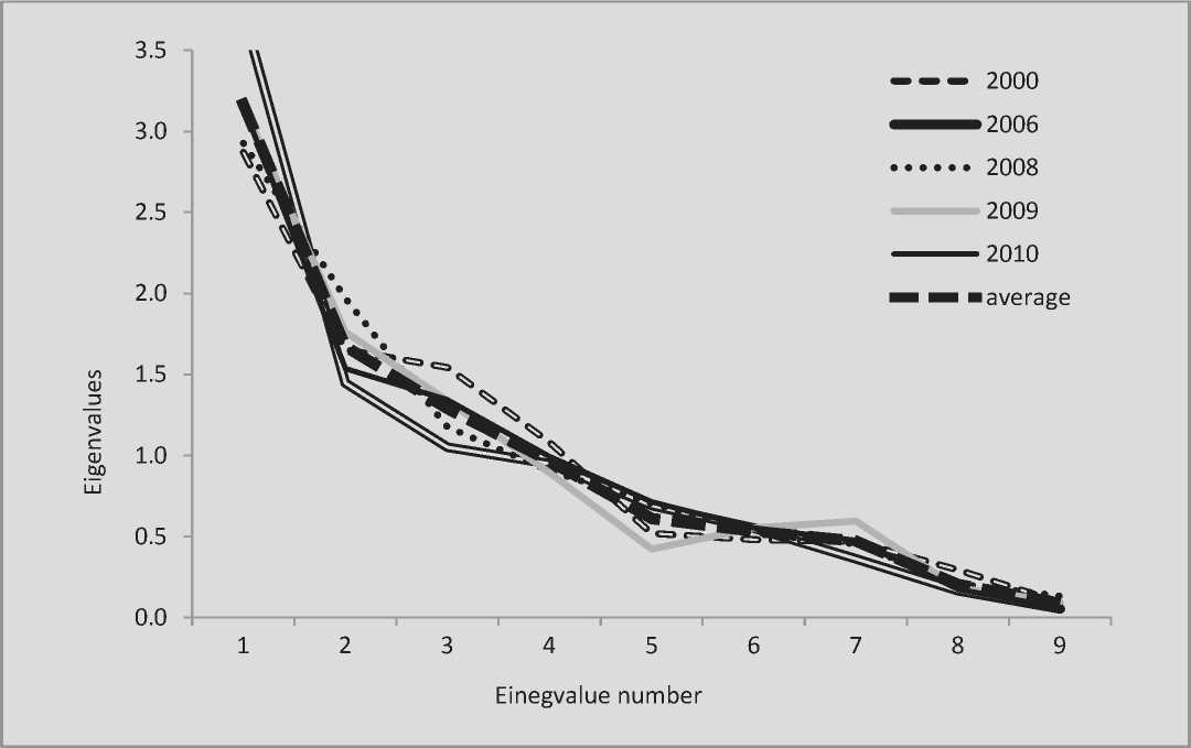
which, amid the unchanging system structure are caused by both changes in the situation and random errors. PCA based on different eigenvector and values different for every time point describes the unchanging structure of the system. Consequently, the eigenvalues and eigenvectors will serve as a signal which needs to be detected from noisy data according to available implementations. The assumption that input data variation of eigenvalues have a common trend is illustrated in Figure 1 which presents the eigenvalues arranged in descending order for different observations.

The average value of the values under review clearly demonstrates the trend (signal) and its random deviation. It is the value averaging that is used in astrophotography for noise suppression. The averaging is based on assumptions that the nature of noise is completely random. Consequently, random deviations from actual data values will continue to decline as the number of observations increases.

Averaging for eigenvectors cannot be used as they are detected by PCA defined accurate to its direction, in contrast with the eigenvalues determined uniquely. The average factor weight value of variables depends on vector direction and cannot uniquely characterize the signal. Therefore, based on eigenvectors calculated for different observations (arranged in descending order of eigenvalues) it is necessary to coordinate the directions of eigenvectors to identify random and non-random components of these vectors and determine coordinate values of nonrandom variables.

The author does not consider a nonrandom (i.e. significant) contribution of a variable in the structure of the main component as a greater value of the rotation weight factor, like in factor analysis, but the invariance of factor weight disturbances (for different observations), the peculiar feature of which is the value of signal-to-noise ratio determined by the ratio of the average value of a variable (signal) and standard deviation (noise). If this ratio is above the threshold value, the variable is considered non-random and significant. If this ratio is not fulfilled, the variable characterizes the noise component of the signal and is not further considered. To check this condition it is necessary to coordinate the directions of eigenvectors based on a criterion. After determining the significant variables they, just like in factor analysis, will be involved in further observation, the insignificant variables are zeroed. A detailed description of the algorithm is presented in [7, 8].

Calculation of integrated indicator quality of life

The author illustrates the algorithm for calculating the integrated indicators of the quality of life in constituent entities of the Russian Federation. The choice of variables and dividing them into blocks are beyond the considered discussion. Therefore the author can use the list of variables (Tab. 1) from the study by M.A. Isakin [5]. The integral indicator of the quality of life is calculated on the basis of three systems of indicators reflecting the integrated categories of the quality of life: the level of population’s welfare, population quality and social quality. The model of the integrated indicator of the quality of life was developed by professor S.A. Aivazyan [1, 2]. The author has used a permanent set of 36 variables [5] for a long time. The author replaces the missing publicly unavailable data with similar to them (highlighted in Table 1). For example, variables 36 and 37 replaced the missing variable “number of suicides per 100.000 people”. All variable values are taken from Rosstat reference books6.

Table 1. Variables for calculating the integrated indices of the quality of life

Block 1: Population’s welfare
1	Pre capita GDP–living wage ratio, units
2	Per capita income purchasing power relative to living wage, %
3	Share of people with incomes below living wage, %
4	The ratio of average income of the richest 20% to the poorest 20% (R\P 20)
5	Number of cars per 1 000 people
6	Share of families on waiting lists for housing, %
7	Total area of housing resources per resident (m²/10 people)
8	Share of dilapidated housing, %
9	Public road density (km/10,000 km²)
Block 2: Population quality
10	Life expectancy at birth, years
11	Mortality rate, infant (per 1,000 live births)
12	Population growth rate, per 1,000 people
13	Deaths caused by communicable, parasitic diseases and TB per 100,000 people
14	Deaths caused by neoplasms per 100,000 people
15	Deaths caused by cardiovascular diseases per 100,000 people
16	Deaths caused by respiratory diseases per 100,000 people
17	Deaths caused by digestive system diseases per 100,000 people
18	Incidence of injuries, intoxication and other external causes per 100,000 people
19	Number of disabled people per 1,000 people
20	Incidence of congenital anomalies per 1,000 people
21	Specialists with higher education employed in economy, %
22	Labor force productivity (GRP per average annual number of employed in economy, thousand rubles/person)
23	Graduates from higher and vocational educational institutions per 1,000 people
Block 3: Social quality
24	Unemployment, %
25	Employers engaged in harmful and hazardous working conditions in the average annual number of employed in economy, %
26	Number of employees injured at work resulting in death or loss of earning capacity for 1 or more days per 1,000 employees
27	Net migration per 10,000 people
28	Intentional homicides per 100,000 people
29	Incidence of intentional infliction of grievous bodily harm per 100,000 people
30	Incidence of rape per 100,000 people
31	Incidence of robbery and theft per 100,000 people
32	Incidence of larceny or embezzlement per 100,000 people
33	Number of registered with drug and substance abuse per 100,000 people
34	Number of registered with alcohol abuse per 100,000 people
35	Number of infected with TB per 100,000 people
36	Mortality from external causes per 100,000 people
37	Number of people with mental disorders per 100,000 people

Missing data imputation is a vulnerable point of the integral characteristics calculation technique. A number of observations largely eliminate this problem. Single missing values are restored by linear interpolation of the available neighboring values; if indicators for a number of years are missing they are supplemented by their average values by federal okrug to which the reporting entity of the Russian Federation belongs.

Further, the set of input variables is unified by the following rules. If the initial indicator is related to the analyzed integral quality feature by uniform dependence, their putting to the interval [0, 1] will transform the variables xij for each time point of observation according to the rule:

a_ij = s_j + ( - 1 ) ^sj

x_ij - m_j

⋅

Mj-mj where sj = 0 if the optimal value of the jth index is maximum and sj = 1 if the optimum value of jth index is minimal, mj – minimum value of the jth index for the whole sample (global minimum), Mj – maximum value of jth index for the whole sample (global maximum).

In case where there is another optimal (not minimum or maximum) index value, the following formula is used:

⎜⎛ aij =, -⎝

xij

opt x_j

max( (M j - xj^opt ),(xj^opt - mj. ))

Among the listed variables, variab

5, 7, 9, 10, 12, 21, 22, 23 are related to the calculated characteristic by the monotonic increasing dependence, when the optimal jth value is maximum. The remaining indicators, except for variable 27, the optimal index value is minimal. For variable 27 “net migration” xjopt = 0, j=27. The value corresponds to the situation where the number of migrants from the region coincides with the number of entrants which, according to the author, is a precondition for a better quality of life in the region.

Table 2 shows the determination of empirical eigenvalues as the average value of eigenvalues of standardized data covariance matrix for different observations of the first block.

The determination of the 3rd empirical principal components obtained by determining significant and insignificant variables of homonymous principal components, is presented in Table 3 . It is necessary to maximize the sum SNR for all variables, which is calculated as the ratio of the calculated average value of factor weights to standard deviation.

All together, 9 options need to be considered, which maximize the calculated SNR for each variable. If the signs of the first variable are identical, the average value of factor weights is maximum and the variation of their values is minimal, consequently, SNR for the variable is maximum. In this case there

Table 2. Determination of empirical eigenvalues for Block 1

Observation	Eigenvalues
Observation	1	2	3	4	5	6	7	8	9
2007	3.38	2.02	1.03	0.87	0.61	0.48	0.30	0.27	0.04
2008	3.41	2.07	0.95	0.87	0.65	0.48	0.29	0.22	0.05
2009	3.24	2.08	0.97	0.89	0.66	0.55	0.32	0.28	0.03
2010	3.25	1.98	1.14	0.82	0.67	0.49	0.33	0.29	0.03
2011	3.26	2.03	1.25	0.73	0.57	0.52	0.35	0.25	0.04
2012	3.30	2.00	1.30	0.73	0.60	0.48	0.34	0.21	0.03
2013	3.42	2.00	1.21	0.77	0.59	0.50	0.27	0.21	0.03
2014	3.43	2.15	1.27	0.65	0.51	0.47	0.28	0.20	0.03
Empirical eigenvalues	3.34	2.04	1.14	0.79	0.61	0.50	0.31	0.24	0.03

Table 3. Determination of the 3rd empirical principal component from Block 1

Coordination of directions of the 1st variable 3 Variables Principal component 1 2 3 4 5 6 7 8 9 2007 -0.07 -0.10 0.26 0.38 0.08 -0.21 0.67 -0.28 -0.44 2008 -0.05 0.19 0.04 -0.14 -0.33 -0.18 -0.41 0.20 0.77 2009 -0.16 0.22 0.19 -0.06 -0.49 -0.20 -0.24 0.04 0.74 2010 -0.17 0.22 0.24 -0.06 -0.37 -0.25 -0.14 0.16 0.79 2011 -0.24 0.18 0.31 0.07 -0.23 -0.20 0.00 0.21 0.82 2012 -0.25 0.18 0.28 0.07 -0.40 -0.23 -0.03 0.17 0.76 2013 -0.20 0.17 0.20 0.01 -0.47 -0.17 -0.03 0.12 0.79 2014 -0.30 0.14 0.18 0.00 -0.38 -0.22 0.04 0.18 0.79 Average, m -0.18 0.15 0.21 0.03 -0.32 -0.21 -0.02 0.10 0.63 Standard deviation, s 0.09 0.10 0.08 0.16 0.18 0.03 0.32 0.16 0.43 SNR 2.10 1.47 2.51 0.22 1.76 7.94 0.06 0.61 1.45 Sum of SNR by line 18.13 Sum of SNR of the current variables 10.45 Coordination of directions of the 2nd variable 3 Variables Principal component 1 2 3 4 5 6 7 8 9 2007 0.07 0.10 -0.26 -0.38 -0.08 0.21 -0.67 0.28 0.44 2008 -0.05 0.19 0.04 -0.14 -0.33 -0.18 -0.41 0.20 0.77 2009 -0.16 0.22 0.19 -0.06 -0.49 -0.20 -0.24 0.04 0.74 2010 -0.17 0.22 0.24 -0.06 -0.37 -0.25 -0.14 0.16 0.79 2011 -0.24 0.18 0.31 0.07 -0.23 -0.20 0.00 0.21 0.82 2012 -0.25 0.18 0.28 0.07 -0.40 -0.23 -0.03 0.17 0.76 2013 -0.20 0.17 0.20 0.01 -0.47 -0.17 -0.03 0.12 0.79 2014 -0.30 0.14 0.18 0.00 -0.38 -0.22 0.04 0.18 0.79 Average, m -0.16 0.18 0.15 -0.06 -0.35 -0.15 -0.19 0.17 0.74 Standard deviation, s 0.12 0.04 0.18 0.15 0.13 0.15 0.25 0.07 0.12 SNR 1.36 4.33 0.79 0.41 2.60 1.03 0.75 2.44 6.00 Sum of SNR by line 19.70 Sum of SNR of the current variables 15.37 are two current variables for which SNR is not less than the threshold 2.2 SNR value, namely variables x3, x6. The sum of ratios of these variables equals 10.45. If the signs of the second variable are identical (as well as 5th, 8th, and 9th), the sum od SNRs calculated for the applicable variables will equal 15.35. This option gives the maximum sum of the calculated SNR values of the existing variables. Thus, this empirical principal component (EPC) contains four operating (important) variables (highlighted dark in Table 3): x2, x5 x8, x9. Factor weights of these variables in EPC are determined by average weights by year, other EPC variables are zeroed (just like in factor analysis).

After defining all empirical principal components there is the issue of their quantity. PNA usually uses a traditional concept of dispersion informational value which determines the number of principal components l used for calculating the integrated characteristics.

where λi – ith eigenvalue of covariance matrix, 6 — threshold of informational value set a priori (typically 55%). The number of selected principal components should implement the ratio (3). Approaches to assessing the number of principal components according to the required proportion of dispersion explained is always formally applicable, but implicitly they assume that there is no distinction between “sig

“noise” and any pre-specified accuracy makes sense. When dividing data into useful signal and noise the specified accuracy loses its meaning and it is necessary to re-define the concept of informational value. Similar to dispersion informational value according to (3) it is possible to determine SNR informational value for the selected empirical principal components N:

_ S 11 ⁺ S 12 ⁺ ... ⁺ S 1 N

^Y S^NR S 21 + S 22 + ... + S 2 n >

where S1k – sum of SNR values of the operating variables of kth EPC, S2k –sum of SNR of all variables of kth EPC. In contrast to dispersion informational value, SNR informational value cannot logically reach 100%. The informational value of the selected system of features is determined by dispersion and SNR informational values:

7 ^_ T c' T SNR . (5)

The number of EPCs for calculating the composite index should maximize the informational value of the obtained solution, defined by (5).

Table 4 shows all normalized (multiplied by the square root of a corresponding empirical eigenvalue) and direction-coordinated EPC of Block 1. The target weights vector is determined by summing homogeneous variables of the number of empirical principal components chosen according to (5).

Table 4. Empirical principal components of Block 1

EPC №	Empirical eigenvalues	Variables
EPC №	Empirical eigenvalues	1	2	3	4	5	6	7	8	9
1	3.34	0.8	0.9	0.82	-0.75	0.53		0.38	0.31
2	2.04	-0.27	-0.31		0.43	0.43	0.64	0.64	0.64
3	1.14		0.19			-0.37			0.18	0.79
4	0.79			0.31
5	0.61								0.34
6	0.5					0.43			-0.26
7	0.31	0.35	-0.12	-0.24						0.19
8	0.24				0.26			-0.2	0.12
9	0.03		0.14	-0.08	0.08
Weights vector		0.88	0.79	0.81	0.02	1.02	0.64	0.83	1.33	0.98

Table 5. Determination of informational value of the integrated index of Blok 1: population’s welfare

	Number of EPCs
	1	2	3	4	5	6	7	8	9
Sum of SNRs of the k^th EPC	102.2	57.6	19.7	11.3	7.9	10.7	20.9	16.5	100.5
Sum of operating SNRs of the k^th EPC	101.4	55	15.4	4.2	3.4	4.9	16.5	10.8	95.7
Accumulated contribution, SNR informational value	0.99	0.98	0.96	0.92	0.9	0.88	0.87	0.86	0.88
Empirical eigenvalues	3.34	2.04	1.14	0.79	0.6	0.5	0.31	0.24	0.03
Accumulated contribution , dispersion informational value	0.37	0.6	0.72	0.81	0.9	0.94	0.97	1	1
Total informational value	0.37	0.58	0.69	0.75	0.8	0.82	0.85	0.85	0.88

Table 5 gives an example of determining the informational value of the integrated index of Block 1. When considering all 9 EPCs informational value is maximum and equals approximately 88%. Therefore, to calculate the integrated index of this block it is necessary to use all of EPCs. The more variables describe the system, the smaller their relative number involved in the compilation of the composite index. The author selects 11 EPCs out of 14

for Block 2, 10 EPCs out of 14 for Block 3. (In another case, 21 EPCs were selected in the system described y 51 variables).

The weight of blocks is determined in proportion to the calculated operating SNR values of this block (Tab. 6), which is similar to that of the proportional strength of the received signal. Block 3 “Social quality”, which contains 14 variables is less important than Block 1 “population’s welfare”, which has 9 variables. Block 2 “Population quality”, which includes 14 variables is the most significant. The significance of population quality is higher than that of population’s welfare and social quality.

Table 6. Block weights

Block

Sum of operating SNRs

307.4

397.7

254.3

Block’s weight

0.32

0.41

0.27

Appendix provides the calculated integrated indices of the quality of life of constituent entities of the Russian Federation in 2007– 2014 taking into account the block weights defined in Table 6. The author presents forecast values for 2015. The value integrated index according to the international practice are normalized relative to values of 2007. The “zero” value has minimum value of the integrated index of the quality of life (IIQL) for 2007 (for Republic of Tuva), 100 is the maximum IIQL value in 2007 (for Moscow). Different Federal districts (FD) are highlighted.

Figure 2 demonstrates the consistency of the technique: it shows changes in the calculated IIQL for some constituent entities of the Russian Federation. The ratio of the calculated characteristics matches the expected figure: Moscow shows indisputable

Figure 2. Integrated characteristics of the quality of life of some constituent entities of the Russian Federation for 2007–2015

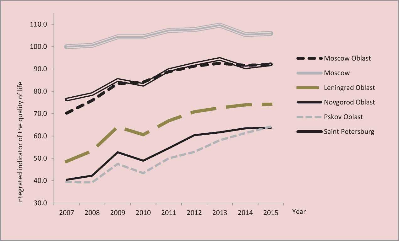
ccessible leadership, Saint-Petersburg and the Moscow Oblast are almost equal in terms of the quality of life, but differ significantly with the capital city, Novgorod and Pskov are the outsiders (not only among the mentioned subjects, but in Russia generally).

Consistently, the highest IIQL indices on the entire interval of observations are demonstrated by regions of the North Caucasian Federal district. It should be noted that 20 indices out of 37 reflect human physiological well-being, which explains (together with the peculiarities of national statistics) the outstanding figures in the republics of North Ossetia, Ingushetia, Chechnya, Dagestan, etc. In these regions risk of illnesses, deaths or criminal violence is lower; the population is not much involved in the process of social production. Life expectancy in Ingushetia is the highest in Russia and, in particular, it is 10 years higher than in the Novgorod Oblast. Taking into account this fact, low GRP and high level of unemployment in the regions of the North Caucasian Federal district do not seem very significant when evaluating IIQL – it is more preferable to live longer and work less rather than vice-versa.

Table 7 shows the average rating for the whole observation period for groups of leaders and outsiders by IIQL. These groups vary slightly by year. The leaders are Moscow, Saint Petersburg, republics of the North

Caucasian Federal district, the Khanty-Mansi and Yamalo-Nenets Autonomous okrugs, Republic of Tatarstan, and some southern regions: the Belgorod, Voronezh, Rostov oblasts, and Stavropol Krai. The last on this list are mostly the regions of the Siberian and Far Eastern Federal districts – 14 entities out of 20 listed, two from the Northwestern Federal district (the Novgorod and Pskov oblasts) and the Volga Federal district (Mari El Republic and Perm Krai). The very last position is permanently occupied by the Republic of Tuva.

Table 8 presents the characteristics of the calculated indices of the quality of life for the whole observation period and the forecast for 2015. The highest differentiation in the quality of life is observed in the Siberian (dispersion coefficient – 29.3) and the Far Eastern Federal districts (dispersion coefficient – 22) with predominant resource-based economy, the lowest – in the North Caucasian Federal district (dispersion coefficient – 7.8). In all Federal districts, the average value of the integrated index of the quality of life during the period under review increased (which is also confirmed by subjective feelings), and differentiation decreased.

However, the differentiation of constituent entities remains significant ( Tab. 8 ), and to overcome it is required to make right management decisions.

It is interesting to compare the obtained IIQL values with the results obtained in

Table 7. Leaders and outsiders by integrated index of the quality of life for 2007–2015

No.	RF constituent entity	Average rating	RF constituent entity	Average rating
1	Moscow	1.00	Khabarovsk Krai	63.67
2	Republic of North Ossetia-Alania	2.56	Novgorod Oblast	65.67
3	Saint Petersburg	3.78	Ivanovo Oblast	66.00
4	Belgorod Oblast	4.33	Republic of Khakassia	67.00
5	Moscow Oblast	5.78	Primorsky Krai	67.33
6	Republic of Ingushetia	7.67	Magadan Oblast	68.22
7	Kabardino-Balkar Republic	7.67	Altai Krai	68.44
8	Republic of Tatarstan	8.44	Mari El Republic	69.89
9	Khanty–Mansi Autonomous Okrug – Yugra	8.56	Perm Krai	70.67
10	Yamalo-Nenets Autonomous Okrug	9.11	Kurgan Oblast	71.56
11	Krasnodar Krai	11.44	Pskov Oblast	71.78
12	Chechen Republic	11.56	Kemerovo Oblast	75.33
13	Karachay-Cherkess Republic	13.78	Zabaykalsky Krai	77.11
14	Stavropol Krai	14.78	Republic of Buryatia	77.44
15	Republic of Adygea	15.11	Chukotka Autonomous Okrug	78.33
16	Republic of Dagestan	15.44	Amur Oblast	78.44
17	Lipetsk Oblast	17.00	Republic of Altai	78.56
18	Murmanks Oblast	17.44	Irkutsk Oblast	79.11
19	Voronezh Oblast	19.89	Jewish Autonomous Oblast	82.00
20	Rostov Oblast	20.22	Republic of Tuva	83.00

Table 8. Characteristics of indices of the quality of life by federal districts

Federal district The whole observation period 2014 Average value Standard deviation Dispersion coefficient, % Average value Standard deviation Dispersion coefficient, % Central 69.6 13.8 19.9 76 11.4 15 Northwestern 63.9 12.5 19.6 71.1 8.6 12 Southern 68.4 10.6 15.4 74.9 9.3 12.5 North Caucasian 79.4 6.2 7.8 84 5.4 6.4 Volga 64.2 9.6 15 69.5 7 10.1 Ural 68.6 11.6 17 72.4 12.2 16.8 Siberian 49.8 14.5 29.2 55.2 12.2 22.2 Far Eastern 52.3 11.5 22 59.3 9.7 16.4 Russia 64 14.8 23.2 69.8 12.6 18.1 ere IIQL for 2012 was calculated using the method proposed by S.A.

Aivazyan. The authors of [10] believe that

“rating compiled using this method helps determine the socio-economic policy priorities at the regional level”. However, careful examination of the obtained results is puzzling. Stavropol ranks 76th, which is close to Tuva with higher rating – 75. The Leningrad oblast with a 63 rating is located between Zabaykalsky Krai region (62), Sakhalin (64), Kalmykia (65) and Yakutia (66). The neighboring Novgorod and Pskov oblasts with the similar situation have a dramatic gap in estimates: 29 for Novgorod and 53 Pskov. Among the regions of the Northwestern Federal district the Leningrad oblast ranks last. Assessments of constituent entities of the Northwestern Federal district seem extremely doubtful; the integrated characteristic cannot be called reliable, it is impossible to correctly “determine the socio-economic policy priorities at the regional level” on its basis.

The source of poor quality of the calculated characteristics may be, in particular, initial data precision which is not taken into account by the traditional method of principal components. The integrated index presented in the current study of resilient relative to input data and is free from gross errors similar to those described above.

Conclusion

The paper reviews the compilation of latent integrated characteristics of changes in the quality system based on recorded statistical measurements. Based on the algorithm of compiling integrated characteristics with identifying non-random components of principal components which characterize the structure of the reviewed system the author identifies the integrated index of the quality of life in constituent entities of the Russian Federation in 2007–2014. During the period under review, the quality of life in all regions improved, the differentiation within the districts decreased. However, the differentiation of constituent entities and federal districts in Russia remains high and in order to overcome it, it is necessary to make right management decisions.

The proposed method can be used to calculate integrated estimates of changes in the quality of any socio-economic system, including calculation of the integrated assessment of the quality of life of constituent entities and municipal formations of the Russian Federation. The results of applying the method of compiling integrated characteristics of quality system changes should be further analyzed using broad social system measurement base recorded by Rosstat, rather than ion terms of a limited set of qualitative input variables.

Integrated indices of the quality of life in constituent entities of the Russian Federation in 2007–2014 (estimates for 2015)

No.	RF constituent entity	2007	2008	2009	2010	2011	2012	2013	2014	2015
1	2	3	4	5	6	7	8	9	10	11
1	Belgorod Oblast	75.9	79.3	83.7	83.8	86.5	92.0	93.3	93.7	94.8
2	Bryansk Oblast	51.1	53.0	59.9	57.4	60.8	64.8	65.6	66.1	66.4
3	Vladimir Oblast	50.3	54.9	61.2	60.3	63.8	66.3	68.0	65.6	65.0
4	Voronezh Oblast	63.9	65.4	68.9	67.9	73.5	79.5	80.3	80.6	79.6
5	Ivanovo Oblast	44.3	49.7	51.4	49.8	54.5	58.4	61.5	61.5	60.1
6	Kaluga Oblast	56.9	60.3	65.9	64.6	70.5	72.7	73.4	74.6	75.0
7	Kostroma Oblast	53.0	54.2	58.7	58.2	60.0	65.9	68.6	68.9	70.4
8	Kursk Oblast	55.9	60.8	66.3	68.3	69.8	75.7	78.2	76.6	77.8
9	Lipetsk Oblast	66.7	66.4	71.4	71.5	75.3	78.9	81.5	82.3	81.0
10	Moscow Oblast	70.2	75.9	83.5	84.1	88.8	91.3	92.5	91.6	92.0
11	Oryol Oblast	57.2	62.7	66.4	63.4	69.9	72.5	75.7	75.1	76.3
12	Ryazan Oblast	57.1	62.4	67.8	66.8	71.7	73.4	77.4	75.7	75.8
13	Smolensk Oblast	45.1	50.2	56.3	55.0	61.0	64.2	68.8	69.5	71.2
14	Tambov Oblast	58.8	62.0	65.3	65.2	68.0	69.8	74.7	72.1	73.3
15	Tver Oblast	42.3	46.0	52.9	50.4	56.4	61.2	64.8	63.7	65.6
16	Tula Oblast	44.0	49.4	58.0	58.0	63.8	67.0	66.6	68.4	68.1
17	Yaroslaavl Oblast	54.7	59.8	66.4	63.6	68.2	69.6	71.9	77.2	77.6
18	Moscow	100.0	100.6	104.4	104.4	107.3	107.6	109.7	105.4	105.9
19	Republic of Karelia	48.9	52.5	57.2	53.0	59.2	61.9	66.3	63.8	65.8
20	Komi Republic	49.8	52.8	56.9	55.3	61.3	64.4	67.6	67.8	70.4
21	Arkhangelsk Oblast	49.3	53.0	59.0	54.5	60.2	63.1	63.5	65.6	66.4
22	Nenets Autonomous Okrug	38.0	50.7	55.1	50.9	57.3	66.5	62.9	71.5	68.6
23	Vologda Oblast	53.6	54.9	57.2	52.1	58.6	63.3	66.7	69.1	71.6
24	Kaliningrad Oblast	60.3	61.5	69.4	70.0	76.5	80.2	81.1	77.7	79.3
25	Leningrad Oblast	48.6	53.4	64.1	60.6	66.8	70.8	72.6	73.9	74.2
26	Murmansk Oblast	67.2	68.3	73.2	75.8	74.5	77.7	82.6	77.5	79.0
27	Novgorod Oblast	40.4	42.3	52.7	49.0	54.5	60.3	61.7	63.4	63.7
28	Pskov Oblast	39.4	39.2	47.5	43.4	50.0	52.9	58.1	61.3	64.2
29	Saint Petersburg	76.3	78.8	85.1	83.0	89.5	92.3	94.5	90.7	92.1
30	Republic of Adygea	60.8	64.9	72.9	71.1	79.3	83.2	85.4	84.9	83.5
31	Republic of Kalmykia	47.6	51.2	56.4	49.4	57.7	61.2	62.5	62.4	62.4
32	Krasnodar Krai	67.8	71.2	78.6	76.3	77.4	82.5	86.3	84.9	85.3
33	Astrakhan Oblast	47.3	51.2	57.2	54.8	59.9	63.3	67.9	67.7	69.2
34	Volgograd Oblast	59.9	61.5	63.2	62.6	64.8	65.7	69.1	70.9	72.6
35	Rostov Oblast	63.1	66.2	71.6	70.1	71.8	76.1	78.8	78.5	80.6
36	Republic of Dagestan	68.8	71.0	72.4	73.0	77.4	79.2	78.6	81.3	82.5
37	Republic of Ingushetia	81.3	86.2	83.8	81.6	81.4	84.7	86.6	80.2	83.0
38	Kabardino-Balkar Republic	76.2	82.3	81.4	79.5	81.3	84.2	85.8	84.6	87.3
39	Karachay-Cherkess Republic	69.2	72.9	76.5	74.9	76.6	79.0	82.2	82.1	84.4
40	Republic of North Ossetia-Alania	83.6	81.7	86.3	87.5	88.5	93.4	94.1	95.7	96.7
41	Chechen Republic	74.6	77.9	80.4	81.9	79.4	78.7	81.6	83.0	79.6

End of Appendix

42	Stavropol Krai	67.4	69.3	72.4	74.6	77.0	80.9	85.3	80.8	81.2
43	Republic of Bashkortostan	64.0	66.4	69.1	67.4	71.3	73.3	75.1	72.2	72.6
44	Mari El Republic	41.8	43.2	52.3	47.3	51.2	54.5	57.7	61.4	61.6
45	Republic of Mordovia	61.0	64.0	66.3	65.5	67.7	69.8	71.6	72.3	71.7
46	Republic of Tatarstan	72.1	74.8	78.0	78.0	81.6	86.0	87.2	85.2	86.4
47	Udmurt Republic	47.8	51.5	57.3	57.8	61.7	66.0	68.1	63.1	64.3
48	Chuvash Republic	47.0	50.2	57.0	52.8	57.7	61.5	62.6	63.9	64.8
49	Perm Krai	40.4	44.5	48.2	46.6	51.8	56.5	60.4	60.4	62.2
50	Kirov Oblast	46.8	49.3	55.4	51.5	56.0	59.1	61.6	64.2	64.3
51	Nizhny Novgorod Oblast	52.2	57.1	63.5	62.6	68.2	71.6	75.3	74.6	74.4
52	Orenburg Oblast	52.6	53.7	58.6	58.5	61.1	63.4	65.6	63.7	63.5
53	Penza Oblast	61.5	64.1	69.4	67.8	72.7	78.1	78.2	75.1	75.5
54	Samara Oblast	64.9	64.8	64.4	65.3	69.1	72.5	71.8	73.8	72.3
55	Saratov Oblast	59.8	63.0	65.4	65.9	67.7	71.0	73.8	73.4	73.8
56	Ulyanovsk Oblast	57.5	61.3	65.4	63.1	66.6	71.9	70.7	70.2	69.9
57	Kurgan Oblast	44.6	45.7	49.7	48.0	51.9	54.1	56.1	54.2	54.2
58	Sverdlovsk Oblast	57.6	58.8	60.7	62.2	64.1	66.8	70.9	71.3	72.2
59	Tumen Oblast	64.0	66.4	66.6	70.2	75.1	78.5	73.4	71.6	69.2
60	Khanty–Mansi Autonomous Okrug – Yugra	74.1	76.5	79.0	78.1	81.3	84.8	86.6	85.2	86.4
61	Yamalo-Nenets Autonomous Okrug	71.1	76.2	80.9	78.3	79.1	81.1	85.9	86.5	89.0
62	Chelyabinsk Oblast	56.4	58.7	61.6	60.6	63.1	64.5	68.0	65.9	68.2
63	Altai Republic	37.8	38.6	40.4	39.4	45.3	48.4	48.3	49.6	49.4
64	Republic of Buryatia	37.3	37.9	42.5	42.8	45.3	48.9	54.9	50.7	52.4
65	Tuva Republic	0	6.7	9.8	8.1	14.8	14.0	20.5	24.9	26.8
66	Republic of Khakassia	47.7	48.8	50.5	50.8	52.4	53.3	59.0	60.2	63.1
67	Altai Krai	46.3	49.3	51.8	48.2	53.2	54.8	58.6	55.6	56.0
68	Zabaykalsky Krai	34.8	37.3	45.7	40.0	46.0	48.6	50.3	54.7	55.7
69	Krasnoyarsk Krai	52.7	53.6	55.2	55.5	59.2	61.2	63.1	63.3	64.7
70	Irkutsk Oblast	38.4	39.4	39.2	38.4	41.2	453	46.2	46.5	48.2
71	Kemerovo Oblast	38.8	41.9	45.3	39.8	46.2	49.1	53.1	53.2	57.0
72	Novosibirsk Oblast	52.5	57.1	61.0	61.7	65.2	67.3	69.5	69.1	69.3
73	Omsk Oblast	53.6	57.9	61.3	61.9	67.3	68.2	66.1	64.2	63.1
74	Tomsk Oblast	61.3	61.1	61.8	63.7	68.2	70.2	72.6	70.5	71.1
75	Sakha (Yakutia) Republic	55.9	54.0	57.7	55.8	60.8	64.3	67.0	69.7	70.9
76	Kamchatka Krai	59.2	62.3	66.4	63.1	64.8	69.0	71.9	71.1	73.2
77	Primorsky Krai	41.4	45.1	51.9	50.9	52.6	57.7	58.9	61.4	63.2
78	Khabarovsk Krai	44.2	45.9	52.5	52.1	54.6	60.0	63.3	60.9	63.8
79	Amur Oblast	35.6	33.9	38.6	36.6	39.9	45.5	52.8	55.5	58.2
80	Magadan Oblast	40.6	38.6	50.5	48.9	57.3	57.8	64.1	60.4	61.3
81	Sakhalin Oblast	45.2	47.0	51.0	51.4	55.6	58.2	64.5	64.2	66.1
82	Jewish Autonomous Oblast	26.3	32.3	34.6	31.2	31.8	38.0	42.2	39.4	44.1
83	Chukotka Autonomous Okrug	32.2	40.7	44.1	34.2	48.7	47.8	45.8	51.1	52.0

Список литературы Building an integral measure of the quality of life of constituent entities of the Russian Federation using the principal component analysis

Ajvazjan S.A. Integral'nye indikatory kachestva zhizni naselenija: ih postroenie i ispol'zovanie v social'no-jekonomicheskom upravlenii I mezhregional'nyh sopostavlenijah . Moscow: CJeMI RAN, 2000. 56 p..
Ajvazjan S.A. Rossija v mezhstranovom analize sinteticheskih kategorij kachestva zhizni naselenija. Chast' I. Metodologija analiza i primer ee primenenija . Mir Rossii , 2010, volume 10, no. 4, pp. 59-96..
Ajvazjan S.A., Stepanov V.S., Kozlova M.I. Izmerenie sinteticheskih kategorij kachestva zhizni naselenija regiona i vyjavlenie kljuchevyh napravlenij sovershenstvovanija social'no-jekonomicheskoj politiki (na primere Samarskoj oblasti i ee municipal'nyh obrazovanij) . Prikladnaja Ekonometrika , no. 3(19), 2009, pp.18-84..
Gajdamak I.V., Hohlov A.G. Modelirovanie integral'nyh pokazatelej kachestva zhizni naselenija juga Tjumenskoj oblasti. . Vestnik Tjumenskogo gosudarstvennogo universiteta , 2009, no. 6, pp. 176-186..
Isakin M.A. Modifikacija metoda k-srednih s neizvestnym chislom klassov . Prikladnaja Ekonometrika , 2006, issue 4, pp. 62-70..
Zadesenec E.E., Zarakovskij G.M., Penova I.V. Metodologija izmerenija i ocenki kachestva zhizni naselenija Rossii . Mir izmerenij , 2010, no. 2, pp. 37-44..
Zhgun T.V. Vychislenie integral'nogo pokazatelja jeffektivnosti funkcionirovanija dinamicheskoj sistemy na primere integral'noj ocenki demograficheskogo razvitija municipal'nyh obrazovanij Novgorodskoj oblasti . Vestnik NovGU. Seriya: fiziko-matematicheskie nauki , 2013, no. 75, volume 2, pp. 11-16..
Zhgun T.V. Postroenie integral'noj harakteristiki izmenenija kachestva sistemy na osnovanii statisticheskih dannyh kak reshenie zadachi vydelenija signala v uslovijah apriornoj neopredelennosti . Vestnik NovGU. Seriya: Tekhnicheskie nauki , 2014, no. 81, pp.10-16.
Zhgun T.V. Issledovanie formal'nyh metodov postroenija latentnoj harakteristiki kachestva system . Vestnik NovGU. Seriya: fiziko-matematicheskie nauki , 2014, no 80, pp.13-19..
Molchanova E.V., Kruchek M.M., Kibisova Z.S. Postroenie reitingovykh otsenok sub"ektov Rossiiskoi Federatsii po blokam sotsial'no-ekonomicheskikh pokazatelei . Ekonomicheskie i sotsial'nye peremeny: fakty, tendentsii, prognoz , 2014, no, 3 (33), pp. 196-208. Available at: http://esc.isert-ran.ru/article/539/full..
Handbook on Constructing Composite Indicators: Methodology and User Guide. OECD Publication. Paris CEDEX 16, 2008. 162 p.
Strizhkova L.A., Zlatoverhovnikova T.V Kachestvo zhizni v rossijskih regionah (dinamika, mezhregional'nye sopostavlenija) . Ekonomist , 2002, no. 10, pp. 67-76..
Strizhkova L.A., Zlatoverhovnikova T.V. Integral'nyi indikator kachestva zhizni naseleniya -IIKZh (sravnitel'naya kharakteristika regionov Rossii) . Upravlenie obshchestvennymi ekonomicheskimi sistemami , 2012, no. 2(2)..
Hightower W.L. Development of an Index of Health Utilizing Factor Analysis. Medical Care, 1978, no. 16, pp. 245-255.
Krishnan V. Constructing an Area-based Socioeconomic Index: A Principal Components Analysis Approach. Early Child Development Mapping Project (ECMap), Community-University Partnership (CUP), Faculty of Extension, University of Alberta, Edmonton, Alberta T5J 4P6, CANADA.
Lindman C., Sellin J. Measuring Human Development. The Use of Principal Component Analysis in Creating an Environmental Index. University essay from Uppsala University, Uppsala, 2011, 45 p.
Manly B. Multivariate Statistical Methods. London: A Primer. Chapman and Hall/CRC, 2004. 208 p.
McKenzie D. J. Measuring Inequality with Asset Indicators. Journal of Population Economics, 2005, volume 18, issue 2, pp. 229-260.
Nardo M., Saisana M., Saltelli A., Tarantola S. Tools for Composite Indicators Building. European Commission, EUR 21682 EN. Joint Research Centre, Ispra, Italy. 2005.
Nicoletti G., Scarpetta S., Boylaud O. Summary Indicators of Product Market regulation with an Extension to Employment Protection Legislation. Economics Department Working Papers NO. 226, ECO/WKP(99)18, 2000.
Saltelli A. Composite Indicators Between Analysis and Advocacy. Social Indicators Research, March 2007, volume 81, issue 1, pp. 65-77.
Saltelli A., Munda G., Nardo M. From Complexity to Multidimensionality:the Role of Composite Indicators for Advocacy of EU Reform. Tijdschrift voor Economie en Management, 2006, volume LI, no. 3.
Somarriba N., Pena B. Synthetic Indicators of Quality of Life in Europe. Social Indicators Research, 2009, volume 94, issue 1, pp. 115-133.
Tarantola S., Saisana M., Saltelli A. Internal Market Index 2002: Technical Details of the Methodology. JRC European Commission. Institute for the Protection and Security of the Citizen Technological and Economic Risk Management Unit I-21020 Ispra (VA) Italy, 2002.
Vyas S., Kumaranayake L. Constructing Socio-Economic Status Indices: How to Use Principal Components Analysis. Oxford University Press, London School of Hygiene and Tropical Medicine, 2006.

Еще

Статья научная