Calculation of complex heat transfer in the liquid circuit of the spacecraft thermal control system based on real topology and thermophysical properties

Introduction. The thermal control system (TСS) is one of the most important systems, which largely determines the design and parameters of the spacecraft (SC) [1]. The characteristics of the TСS have a significant impact on the circuit solutions for the placement of heatgenerating equipment inside the SC, the layout of heatemitting radiation panels, which in turn forms the geometric and weight dimensions of the SC [2; 3].

Priority tasks of modernization and technical improvement of rocket and space technology require the creation and development of appropriate software and algorithmic support for the calculation of all major SC systems, including TСS [4; 5].

The work on creation of thermal mathematical models of TСS, algorithms of calculation allowing forming effective design solutions at various stages of constructing is conducted in this sphere.

At the previous stages of the study, the authors [6; 7] obtained systems of equations for the liquid circuit of the spacecraft TCS in the form of heat balances determined relatively to the temperatures of the specific heat exchange surfaces. Mathematical models and algorithms for determining the complex thermal resistances for LC were

obtained, which significantly simplify the computational procedures for calculating the main characteristics of the TCS.

Statement of the research problem. The aim of this work is to bring the system of heat balance equations of LC TCS [6] to the form that allows to perform numerical integration in the algorithm for finding a solution along the length of the middle line of the heat and mass transfer of liquid circuit, taking into account the complex thermal resistances determined by the real topology and thermal properties of the LC. In fact, this means that in the record of equations [6] as the variables should remain the members of the temperature values of the contour and the linear coordinate – integration variable, everything else should be numerically determined by the properties of the real object.

Calculation scheme. Currently designed LC TCS can have different topology, which determines the placement of the basic elements, which forms the final design appearance of the TCS [8–10]. As an example, consider a fragment of the heat transfer circuit in the TCS, which includes a honeycomb panel with a liquid circuit pipe placed on it (fig. 1).

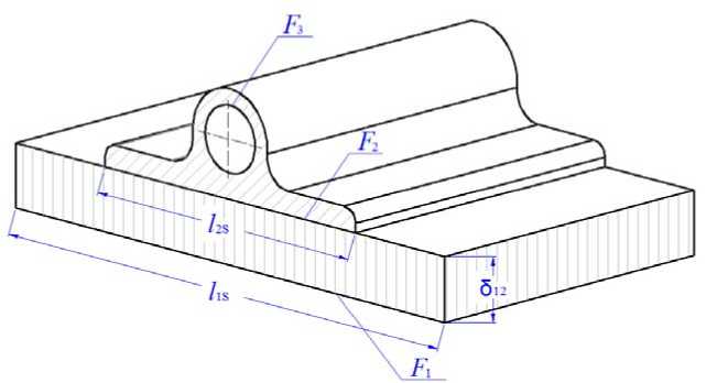
Fig. 1. Calculation scheme of the fragment of the heat transfer circuit

Рис. 1. Расчетная схема фрагмента контура теплопередачи

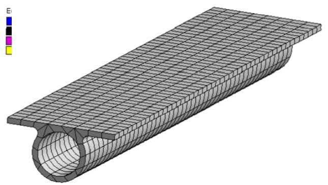
Fig. 2. Finite-element model of the TCS liquid circuit

Рис. 2. Конечно-элементная модель жидкостного тракта СТР

As the initial data, we take the following: the value of the thermal conductivity coefficient for the honeycomb in the transverse direction λ₁₂ = 6 W/m∙К; the width of the honeycomb l _{1 S} = 0.18 m; the width of the heel of the pipe of the liquid circuit l 2 S = 0.02 m; the thickness of the honeycomb δ 12 = 0.03 m; the total length of the liquid circuit l 1 x = 50 m.

This design solution forms three characteristic heat exchange surfaces [11]: the outer surface of the honeycomb panel F 1 , the surface of the heel of the pipe F 2 and the inner surface of the pipe F 3 , which determines, respectively, three isothermal surfaces Т 1 , Т 2 , Т 3 .

For the outer surface of the honeycomb panel corresponding to the isothermal surface Т ₁ at the integration step Δ x_i the area of increment is determined by the expression:

AF„ =A F = A x, ■ l = 0,18 A x ,. (1) 12 i 1 ii 1 S i

For the process of heat transfer between surfaces Т 1 and Т 2 the equivalent thermal resistance R λ12 i can be represented as:

these purposes, the finite element method implemented in the Ansys software package is applicable. Fig. 2 shows the finite-element model of the TCS liquid circuit.

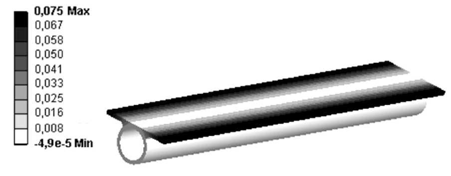
Numerical investigation of temperature fields of the liquid circuit. To solve the problem of definition the thermal resistance across the pipe cross section we use the following boundary conditions: heat flux on the LC flange is 10 W; inner diameter profile – 12 mm, flange width – 20 mm; wall thickness – 2 mm; constant temperature on the inner wall of LC – 0 °C; coefficient of thermal conductivity – 155 W/K∙m. In fig. 3 the results of the stationary calculation for the stated boundary conditions are presented.

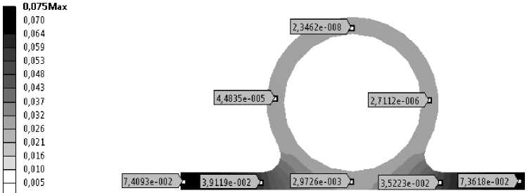
Fig. 3 shows that the maximum temperature drop across the pipe section does not exceed 0.0755 °C, and due to the high thermal conductivity of the LC profile, the drop in the pipe section is negligible. It follows that the thermal resistance for the transverse direction can be defined as:

^R М2 i =

^- 12 ^{A F} 12 i = ¹

§ 12       ^R - 12 i

________ § 12 _________ in I l 2S

^— 12 ■ ^{A x}i ■ ⁽ l 2 S "  ^l 1 S )   1 ¹ 1 S

0.03          , I0.02) 0.068

--in =------; 6.0 ■A x i - (0.02 - 0.18) ( 0.18 J A x i

-^---12^ = — = 14.71 A x (2)

§17         R 12             - 12 i

To define an expression for the equivalent thermal resistance between the isothermal surfaces Т 2 and Т 3 , forming a channel profile, you must also determine the thickness of the equivalent thermal resistance, which in this case requires numerical calculation of the thermal resistance on the lineal meter of LC TCS profile [12]. For

R _=T^=- = °.° ⁷⁵⁵ = 7.55 ■Ю "³ K/W. (3)

^- S ²³     Q 10                             ^{V 2}

To solve the problem of definition the thermal resistance along the cross section of the pipe, the following boundary conditions should be settled: heat flow on the cross section of the end profile of LC 10 W; a constant temperature at the cross section of the opposite end of the profile LC 0 °C; inner diameter profile 12 mm, flange width 20 mm; wall thickness 2 mm; the coefficient of thermal conductivity 155 W/K∙m; length of profile 1m; cross-sectional area profile of LC F = 4.6357∙10-3m2.

Fig. 4 shows the results of stationary calculation of the temperature field for this case.

In this case, the thermal resistance is directly proportional to the length of the section of the profile and is defined as:

^R - S 23 =

A T

Q

l

-■ F

155 ■ 4.6357 ■Ю "³

= 1.39 K/W

— -4,9 e-5 Min

Fig. 3. Results of stationary calculation of the temperature field

Рис. 3. Результаты стационарного расчета поля температур

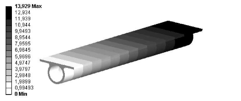
Fig. 4. The results of the stationary calculation of the temperature field for the pipe in the longitudinal direction

Рис. 4. Результаты стационарного расчета поля температур для трубы в продольном направлении

From the comparison of the data it can be seen that the thermal resistance coefficients in the longitudinal and transverse directions differ ~ 200 times. This means that the main direction of heat transfer will be transverse when modeling the TCS. In this case, the longitudinal direction in the first approximation can be neglected.

The above calculations had fixed flange and pipe surface temperatures as boundary conditions. Thus heat transfer from the heat carrier to a wall was not considered. This approach makes it possible to obtain the value of thermal resistance, due only to the mechanism of thermal conductivity [13].

Consider the effect of heat transfer on the value of thermal resistance. To do this, as a boundary condition on the wall of the pipe, we indicate the convective heat exchange with the flow of the coolant. We use the following boundary conditions: heat flow to the LC flange 10W; internal diameter of the profile 12 mm; width of the profile flange 20 mm; wall thickness 2 mm; constant temperature of the coolant flow LC 0 °C; thermal conductivity of the material: 155 W/K∙m; to determine the heat transfer coefficient of the coolant used experimentally obtained the dependence on temperature (fig. 5).

Fig. 6 shows the results of the stationary calculation of the temperature field of the pipe cross-section taking into account the effect of heat transfer.

Analysis of the results. The calculation resulted in temperature fields on the surfaces of the pipe and flange, the maximum temperature difference was 0.168 K. Accordingly, the thermal resistance in this case is 1.68∙10^–2 K/W. Thus, the lowest thermal resistance characterizes the case of heat transfer in the transverse direction without taking into account the convective heat transfer. In this case, the thermal resistance value will be equal to 7.55∙10^-3 K/W.

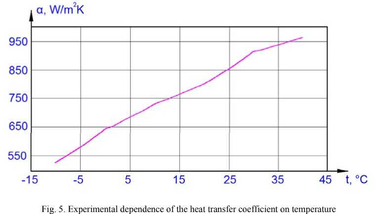
Рис. 5. Экспериментальная зависимость коэффициента теплоотдачи теплоносителя от температуры

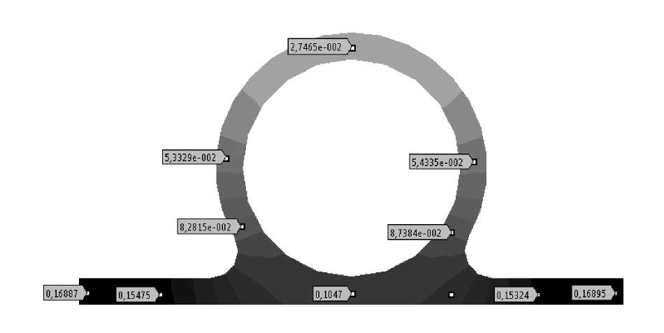
Fig. 6. The results of the stationary calculation of the temperature field of the cross section of the pipe, taking into account the effect of heat transfer

Рис. 6. Результаты стационарного расчета поля температур поперечного сечения трубы с учетом влияния теплоотдачи

Thermophysical parameters of the profile per lineal meter

№	Parameter	Description	Dimension	Value
1	The thermal conductivity of the pipe material of LC	X 23	W/K∙m	155
2	Pipe fladge width	l 2 S	m	0.02
3	The circumference of the pipe	l 3 S = n d 3	m	0.0377
4	Thermal resistance	R X S 23	K/W	7.55∙10-3
5	Heat flow	Q 23	W/m2	10.0

According to the calculation results, see table of thermophysical parameters for heat transfer between surfaces T ₂ and T ₃ and in fig. 1 on the lineal meter of the profile were formed.

The equivalent thickness of the thermal resistance of the pipe is determined by the expression

^T 3 i = T -;

q HP - 0.02 A x i - 137 A x i - ( T, i - T i ) = 0;

8 S 23 =

^X 23 ^- ( ^l 3 S   ^l 2 S ) ^- R X S 23

A Q si = 14.71 A x i - ( T i - T 2 i );

= 0.0326 m.

Thus, the equivalent of the thermal resistance of the thermal conductivity between the surfaces T ₂ and T ₃ has the form

R =        8 S 23         ln Г l^ ) 0.0073

• ^X231   X 23 -A xi - ( I s 3 - I s 2 )     ( l_s 2 ^J     A x, ’

or

• ^X 2 ^{3 -A} F ^{23 i} = — = 137 -A x i         (6)

⁸ 23 i        R X 23 i

For convective heat transfer from a surface T ₃ to a

conditional surface T ₄ , the area increment at the integration step has the form

A F 34i = l 3 s -A x i = 0.0377 A x i            (7)

With zonal heat transfer between isothermal surfaces T₆ - T ₅ , the parameters will be similar to the case of T ₂ - T ₃ : surfaces:

AF65i= 12s 'Axi = 0.02Axi;(8)

biiAF- = -1- = 137Ax;.(9)

865i

Use the following numerical values for the coolant of the liquid circuit LZTK2 (isooctan): mass flow rate of 0.071 kg/sec, heat capacity of 2060 J/ kg∙K, heat transfer coefficient according to the model spills on similar profiles of 600 W/ mxK. Taking into account the values of the determining parameters presented in [6] the system of heat balances for the liquid circuit of the TCS from the south side takes the form:

A S - S ₀ - 0.18 A x i - sin a-e-o- 0.18 A x i x

X T 4 - 14,71 A x i- ( T 1 i - T i ) = 0;

14,71 A x i - (T - ? 2 ,) - 137 A x i ■( T2, - T 3 i ) = 0;

137 A x i ■( T i - T i ) - 22.62 A x i ■( T 3 i - T _{4 1} ) = 0;

A Q , _s = 146.26 - ( T 4 i - T 4 i _{+ 1} ) ;

Q , s = 146.26 - ( T 4 sn - T 4 s 0 ) .

Similarly the balance system on the north side:

• -e - o - 0.18 A x i - T 1 4 + 14.71 A x i - ( T ₂ i - T_u) = 0;

• - 14.71 A x i - ( T_2i - T_1i) + 137 A x i - ( T ₃ i - T ₂ i ) = 0;

  - 137 A x i - ( T ₃ i - T _{2 i} ) + 22.62 A x i - ( T ₄ i - T _{3 i} ) = 0;

T 3 i = T 5 i ;

q HP - 0.02 A x i - 137 A x i- T - T 5i ) = 0;

A Q , Ni = 146.26 - ( T^- T 4 _{1 4}1 );

Q , n = 146.26 - ( T ₄ n 0 - T ₄ Nn ).

Thus, in the presented form, the systems of balance equations of the liquid circuit of the TCS are fully defined and ready for numerical solution. As a result of the solution of systems (10), (11) values of characteristic temperatures of isothermal surfaces of TCS are defined.

Conclusion. In this paper, taking into account the real topology and thermal properties of the LC, the values of equivalent thermal resistances for the characteristic heat transfer sites in the liquid circuit of the spacecraft were obtained numerically. Using these values, the system of heat balances of LC TCS on the characteristic surfaces of constant temperature was led to the form that allows numerical solution: the number of equations corresponds to the number of defined temperatures for the northern and southern panels and is closed through the temperature of the cooling liquid circuit. The system of equations makes it possible to study the thermal state of the SC of non-hermetic design at the stage of preliminary design with variation of operating and design parameters in order to determine the range of performance and the optimal operation under certain efficiency criteria [14–17].