Calculation of the Classic-Curvature and the Intensity-Curvature Term Before Interpolation of a Bivariate Polynomial

Published Online November 2015 in MECS DOI: 10.5815/ijieeb.2015.06.06

Magnetic Resonance Imaging (MRI), Computerized Axial Tomography (CAT), Electroencephalography (EEG) and Magnetoencephalography (MEG) are among the most useful technologies available to study the human brain. For instance, resting-state electroencephalogram signal is very useful for the neurologists, the clinicians and the physicians in order to determine the baseline of the human brain EEG. Time delay neural networks (TDNNs) and probabilistic neural networks (PNNs) trained with nonlinear features (Lyapumov exponents and Entropy) have been demonstrated useful in order to classify electroencephalogram signals (EEG) of the human brain and so to discriminate between normal controls and subjects affected by partial epilepsy [1].

Another work, related to the detection of EEG epileptic spikes has been reported and an application of Linear

Discriminant Analysis (LDA) has been used in order to classify the EEG spikes signals [2]. EEG combined with signal post-processing based on wavelet phase coherence has been employed to study the resting state networks in the human brain in the two conditions of eyes closed and eyes open and the results have shown the predominance of the alpha band in the condition of eyes closed [3]. The aforementioned finding is consistent with previous research results obtained with Magnetoencephalography [4].

MRI, on the other hand, is paramount in imaging, in diagnosing, and in studying abnormalities and diseases of the human brain and is of crucial help in order to the examine the biological and the clinical concomitants of the diseases. The immediate benefit of Magnetic Resonance Imaging is that it helps to discover the existence of a brain tumor and to identify where the brain tumor is exactly located. MRI, as a diagnostic technology, also allows the diagnosis of the type of the tumor and also the identification of the denomination of the cancer pathology, in other words, the classification of the tumor.

Human brain tumors likewise other cancer pathologies are characterized by unregulated cell growth [5]. The unregulated cell growth in cancer is also characterized by the pace at which it takes place. The growth can be slow, but can also be such to determine fast spreading of the tumor cells into the human body.

Therefore, the severity of the disease and the need for a surgery, and/or radiation, chemotherapy, hormone therapy, biological therapy, and targeted therapy needs to be assessed immediately [5]. MRI is one of the most rapid and used technology that can make the aforementioned assessments. More generally, acquisition, processing and retrieval of data related to the patient, yields to interoperability of health related information and is necessary in order to provide effective and efficient healthcare [6]. To this regard, the use of Information Communication Technologies (ICT) and usage of ICT resources is pivotal [6].

The work presented in this paper may frame the two intensity-curvature measurement approaches named: (i) classic-curvature image and (ii) intensity-curvature term before interpolation image [7]; within the context of ICT technologies which aim is to post-process MRI data in order to extract information about the human brain tumor mass, and to help physicians to study and analyze the tumor.

• A.    The Literature

Magnetic Resonance Imaging (MRI) is the most powerful diagnostic technology [8, 9] because allows visualization of the human brain, and more generally of all of the body structures, without side effects, and is employed also to diagnose tumors in the human brain [10, 11]. This paper is concerned with the calculation of the classic-curvature image [12] and the calculation of the intensity-curvature functional term before interpolation image [13-17] using MRI data consisting of a twodimensional image of a human brain affected by a tumor.

• B.    The Technological Effort

To obtain the classic-curvature image and the intensitycurvature term before interpolation image, the calculations demand the computation of the four partial second order derivatives of the model function fitted to the image. The intensity-curvature functional before interpolation image can be calculated on the basis of the classic-curvature image. Both of the aforementioned intensity-curvature measurement approaches [7] descend from the model function used to create the continuum in the MRI data. The second order partial order derivatives, the classic-curvature, and the intensity-curvature term before interpolation were implemented in software and were successfully calculated and visualized with the use of the following computer technology applications: (i) Visual Studio IDE, (ii) jdk-6u-45windows-x64 (Java), (iii) jre-7u71windows-x64 (Java), (iv) the computer Operating System (OS) command prompt and (iv) ImageJ .

Thus, the computational effort of the works herein presented consist into the software implementation of the mathematical procedures outlined in the theory and methods section. The code implementing the mathematical procedure has been tested and debugged successfully and so it was possible to open the command prompt to run the program in order to obtain the intensity-curvature measurement approaches. Last but not the least, ImageJ was used to open and visualize the images derived from the calculations.

• C.    The Scope of the Research

As the theory and methods section will show through the presentation of the mathematical formulation, the intensity-curvature measurement approaches object of study in this paper are: (i) the classic-curvature image, and (ii) the intensity-curvature term before interpolation image; and they were obtained on the basis of the calculation of the first order and second order partial derivatives of the bivariate polynomial model function fitted to the MRI data.

The calculation of the classic-curvature and the intensity-curvature term before interpolation enables us to create two additional domains where is possible to see the human brain data under a different perspective. The classic-curvature images have been object of considerable study [7, 12, 14, 17] and allow to distinguish clearly the brain tumor. Moreover, similarly to the original MRI image, the classic-curvature image shows a clear layout of the tumor and the surrounding brain structures. The original MRI image analyzed together with the intensitycurvature term before interpolation (which is an image also) can provide both research and diagnostic settings with additional and/or complementary information about the human brain structure under study. The main scope of the paper is to study and to introduce in the literature the use of the intensity-curvature term before interpolation. And, to the purpose of introducing the intensity-curvature term before interpolation, a pathological human brain MRI image showing a tumor has been studied.

In order to frame into the literature the works of this research, which recalls works reported earlier [7, 12-17], it is necessary to consider the rationale of the study presented in this paper. So far, no studies have been reported attempting to achieve the characterization of the intensity-curvature term before interpolation. Thus, the rationale of the study herein presented is to characterize the behavior of the intensity-curvature term before interpolation. Therefore, the research presented in this paper is a novelty in the literature.

• II.    Theory and Methods

The mathematical procedure outlined in this paper is based on the process of fitting a bivariate polynomial model function to the image data. The advantage of fitting the model function to the MRI data consists in the creation of the continuity inside the pixels of the image. Thus, the continuity makes it possible to calculate the following properties of the MRI image: (i) the first order partial derivatives, (ii) the second order partial derivatives, (iii) the classic-curvature, and (iv) the intensity-curvature term before interpolation. Thus, there are four second order partial derivatives of the bivariate polynomial model function fitted to the image data because the MRI images are two-dimensional.

The classic-curvature of an image is defined as the sum of the four second order partial derivatives which belong to the Hessian of the polynomial model function fitted to the image data [12]. The intensity-curvature term before interpolation is defined as the integral of the multiplication between the pixel intensity f(0, 0) and the classic-curvature calculated at the origin of the pixel coordinate system ((x, y) = (0, 0)). Both of the classiccurvature and the intensity-curvature term before interpolation fall into the category of intensity-curvature measurement approaches [7].

Therefore, the mathematical method presented in this paper can be a viable option to post-process MRI data in order to obtain intensity-curvature measurement approaches departing from collected MRI images of the human brain. In this section of the paper is reported the entire mathematical procedure used in order to calculate the classic-curvature and the intensity-curvature term before interpolation departing from a bivariate polynomial.

• A.    The Model Function

g(x, y) = f(0, 0) + αг ⋅ а(х3у3 +х2у2) +

α3 ⋅ b(х3у3 +х2у2 )

• B.    The Definition of the Classic-Curvature

у (х, у) =     ( 8 ( , у )) ₊     ⁽ 8 ⁽ 2 ^, у ))

у (х, у) =        ++

( g ( X , У ))        ₍ g ( , У ))

Sy 8х8у

(6ху3 + 2у2) + (6ух3 + 2х2)+

α2 ⋅а [(9у2х2 + 4ух + 1) + (9х2у2 + 4ух + 1)]+

α ⋅b [   (6ху3 + 2у2 ) + (6ух3 + 2х2)+

α    (9у х +4ух+ 1) + (9х у +4ху+ 1)]

To calculate у (0, 0) we substitute x = 0 and y = 0 in equation (9) so to obtain:

у (0, 0) = α2 ⋅ а (0 + 0 + 1 + 1) +

α3⋅b (0+0+1+1) =

(2α2 ⋅ а + 2α3 ⋅ b)                (10)

• C.    First and Second Order Partial Derivatives Respect to the x Variable

^{( ( ( ,} )) _{= α} 2 ⋅а (3х²_у³ + 2ху² + у) +

α3 ⋅ b (3х2у3 + 2ху2 + у)(3)

⁵² ( | ^{( , ))} = α 2 ⋅ а (6ху³ + 2у²) +

α3 ⋅ b (6xy3 + 2у2 )(4)

• D.    First and Second Order Partial Derivatives Respect to the y Variable

  - ⁽ ( , ⁾⁾ = α2 ⋅ а (3у²_х³ + 2ух² + х)+

α3 ⋅ b (3у2х3 + 2ух2 + х)(5)

δ ³ (g(х, у)) δу²

α2 ⋅ а (6ух3 + 2х2) +

α3 ⋅ b (6yx3 + 2х2)

• E.    Second Order Partial Derivative Respect to the x and y Variables

• 52 ( 8- ( , У-)) = α 2 ⋅ а (9у2х2 + 4ух + 1) + 8х 8у        z 4у

α3 ⋅ b (9у2х2 + 4ух + 1)(7)

• F.    Second Order Partial Derivative Respect to the y and x Variables

^{52 ( 6}- ( , ^у _; ⁾⁾ = α2 ⋅ а (9х²у² + 4ух + 1)+

α3 ⋅ b (9х2у2 + 4ху + 1)(8)

• G.    The Calculation of the Classic-Curvature

у (x, y) = (α2 ⋅ а (6xy3 + 2у2) + α3 . b (6xy3 + 2у2 )) +

(α2 ⋅ а (6yx3 +2х2) + α3 . b (6yx 3 + 2х2 )) +

(α2 ⋅ а (9у2х2 + 4ух + 1) + α3.b (9у2х2 + 4ух + 1)) +

(α2 ⋅ а (9х2у2 + 4ух + 1) + α3.b (9х2у2 + 4ху + 1)) =

• H.    The Intensity–Curvature Term Before Interpolation

Е_о (х, у) = ∫ _∫ ,^У(f(0,0) ⋅ у (0,0)) ԁх ԁу=

∫ ∫ ,У(f(0,0) ⋅ (2α2а+ 2α3 b)) dх ԁу= (f(0,0)) ⋅ (2α2а+ 2α3 b) ⋅ ух         (11)

• I.    Steps to Follow to Process the Magnetic Resonance Imaging Data with the Computer Program and the Use of the ImageJ Application

Step 1: Open the Windows OS command prompt.

Step 2: Type cd to change the directory, copy the path of the ‘templateCurvature’ (which is the computer program:  software implementation of the intensity curvature measurement approaches and also the name of the executable used for computing).

Step 3: Paste the path of the ‘templateCurvature’ and press enter.

Step 4: Type ‘templateCurvature’ (the name of the executable) and press enter. Read the instructions given by the computer program over the command prompt (see Fig. 1).

Step 5: From the debug folder, copy the name of the program ‘templateCurvature’ and paste it on the command prompt. Also, have available the file name of the image which has to be processed and type it after the program name leaving a blank in between the program name and the file name of the image (example: templateCurvature blank image name; see Fig. 1). Do not press enter.

Step 6: Type ‘.img’ so to complete the image file name. At this point leave a blank on the command prompt and then, as instructed by the computer program, input sequentially all of the parameters to the computer program so that the image can be processed (see Fig. 1). Hit enter and let the computer program process the image.

Step 7: Open the ImageJ application, click on ‘file’, then click on ‘import’ and select ‘raw’ so to show the original image as it can be seen in Fig. 2.

Step 8: Use of ImageJ. In the ‘Image Type’, select ‘64 bit real’, enter the values of the width and height pixels. The values must correspond to the number of X and Y pixels used as input to the program in step 6 (i.e. X is the height of the image and Y is the width of the image).

Step 9: Use of ImageJ. For this project, the offset to first image must always be set to 0 bytes, the number of images set to 1, and the gap between images set to 0 bytes. Check the box named ‘Little-Endian Byte Order’ and leave unchecked the rest of the boxes. Click OK to open the image.

• J.    The Calculation of the Intensity-Curvature Measurement Approaches

The ten cases studied in this paper have used the same MRI image (see Fig. 2). Thus the computer program implementing the mathematical procedure, in each of the ten cases, was given as input the same number of pixels along the X and Y direction, the same pixel size along the X and Y direction, the same XY rotation angle but different numbers for ‘a’ and ‘b’ constants.

C:\templateCurvature\Debug>templateCurvature

Piease type the image file name Piease make sure that the image format is Analyze 'double': 64 bits real Before running the program, please make sure that the image is padded of 'n >= 0 'number of pixels along X and V Piease enter the number of pixels along the X direction (integer)

Piease enter the number of pixels along the Y direction (integer)

Please enter the pixel size along the X direction (double)

Please enter the pixel size along the У direction (double)

Piease enter the misplacement along the X direction (double) Piease enter the misplacement along the Y direction (double) Please enter the ХУ rotation angle (double) Please enter the a constant (double) Piease enter the b constant (double) Piease enter that 'n >= 0' number of pixels along X and У directions which will pad the image Processing will not be correct if you enter a value of n which is greater than the actual number of pixels along X and Y which was used to pad the image before running the program.

Please type 'n' to scale the Image Data or 'e' to exponentialize the Image Data

0.5 0.5 0.0 -5.0 -7.0 2 n________________________________________________________

Fig.1. The Windows OS command prompt showing the instructions given by the computer program called ‘templateCurvature’. The program asks to the user to input sequentially the following input parameters: (i) the program name: ‘templateCurvature’, (ii) the image file name with extension ‘.img’, (iii) the number of image pixels along the X direction, (iv) the number of image pixels along the Y direction, (v) the pixel size along the X direction, (vi) the pixel size along the Y direction, (vii) the rotational angle, (viii) the ‘a’ constant, (ix) the ‘b’ constant, (x) the number of pixels of the image pad, (xi) the choice between scaling (option ‘n’) and standardization (option ‘e’) of the image data. The computer program requires to swap the order of the number of image pixels along X and Y directions on the command line. The computer program ‘templateCurvature’ is derived from the freeware downloadable at the URL:

• III.    results

The main scope of the paper is to report for the first time in the literature on the behavior of the intensitycurvature term before interpolation. The results presented in this section have been collected when processing MRI data of the human brain in pathological state (tumor MRI). Therefore, it is relevant to open this section of the paper introducing immediately to the reader on the behavior of the intensity-curvature term before interpolation images which are capable to add supplemental information to the MRI image shown in Fig. 2a.

The supplemental information is provided through the change of the appearance of the human brain image as visible in the intensity-curvature term before interpolation images (compare Fig. 2a with Figs. 3, 4 and 5b), which results into the highlight of a specific tumor structure of the tumor MRI.

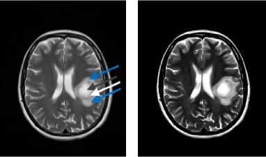
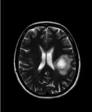
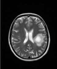
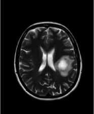
The specific tumor structure is the circular zone surrounding the tumor inner metastasis located at the center of the tumor mass (see circular zone indicated by the white arrow in Fig. 2a). Thus, a different yet informative perspective of the tumor structure is available because of the appearance of the image calculated with the aforementioned intensity-curvature measurement approach and such perspective may have medical value.

(a)                       (b)

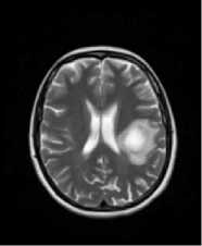
Fig.2. The collected MRI in (a) shows a pathological human brain displaying brain metastases. The image is found in [17]. In (b) the MRI is contrast-brightness adjusted so to highlight three zones indicated in (a) by the arrows: (i) the inner metastasis located at the center of the tumor mass (see gray arrow), (ii) the circular zone surrounding the tumor inner metastasis (see white arrow), and (iii) the outer metastasis surrounding the all tumor mass (see blue arrows). The distinction between (ii) and (iii) will become clear and neatly observable in Figs. 3, 4, 5, 6 and 7, similarly to what can be seen in (b).

It is also due to introduce that the classic-curvature images herein presented display characteristics similar to those of the intensity-curvature term before interpolation images. However, the emphasis is on the intensitycurvature term before interpolation images because of the fact that they are studied for the first time in the literature. The contrast-brightness level of the classic-curvature images and the intensity-curvature before interpolation images shown in this section of the paper was set so to bring out the best possible information content of the images. The contrast-brightness level is a necessity of the images, which otherwise, would not show the potency that allow to highlight the features of the human brain and the tumor mass (see for instance Fig. 2b).

• A. The Classic-Curvature and the Intensity-Curvature Term Before Interpolation Images

As anticipated in the previous section of the paper, the ten cases processed in this work had the same number of pixels along the X and Y directions. The same pixel size along the X and Y directions. The same XY rotation angle. However, each case was given different values of the ‘a’ and ‘b’ constants (thus ten different numbers have been used for the ‘a’ and ‘b’ constants: ten for ‘a’ and ten for ‘b’). The ‘a’ and ‘b’ constants appear in the bivariate polynomial model function in (1), and, consistently with the mathematical procedure, they also appear in the relevant formulae of the theory and methods section of the paper. Five ‘a’ constants and five ‘b’ constants are negative and the remaining five ‘a’ constants and five ‘b’ constants are positive. The images of the classiccurvature and the intensity-curvature term before interpolation are reported in this section of the paper for each of the couples of ‘a’ and ‘b’ constants.

In Fig. 3, Fig. 4, Fig. 5, Fig. 6 and Fig. 7 the image name is xxni00001-0011.img, the number of pixels along the X direction is 320, the number of pixels of Y is 262, the pixels size along the X direction is 1.0mm, the pixels size along Y direction is 1.0mm, the misplacement along X direction is 0.5mm, the misplacement along the Y direction is 0.5mm, the XY rotation angle is 0.0 degrees, and the number of pixels along the X and Y directions used to pad the image is 2. The choice between the scaling (option ‘n’) and the standardization (option ‘e’) of the image data is set to ‘n’. The misplacement along the X and Y directions consists of the re-sampling coordinate (x, y) which is relevant to the formulae reported in the theory section of this paper. Thus, the intensity-curvature measurement approaches: (i) classic-curvature, and (ii) intensity-curvature term before interpolation, which are formulated in the theory section were calculated in this section of the paper with the value (x, y) = (0.5, 0.5).

(c)                         (d)

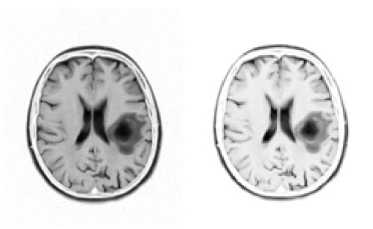
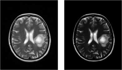
Fig.3. The images in (a) and in (b) were calculated with the ‘a’ constant set to the value of -5.0, and the ‘b’ constant set to the value of -7.0. The images in (c) and in (d) were calculated with the ‘a’ constant set to the value of -7.0, and the ‘b’ constant set to the value of -9.0. In (a) and in (c) are shown the classic-curvature images calculated from the image seen in Fig. 2a, and in (b) and in (d) are shown the intensity-curvature term before interpolation image calculated from the image seen in Fig. 2a. The circular zone surrounding the tumor inner metastasis (which is shown in dark color) is visible in bright color both in the classiccurvature images (a), (c), and in the intensity-curvature term before interpolation images (b), (d).

(a)                             (b)

(c)                             (d)

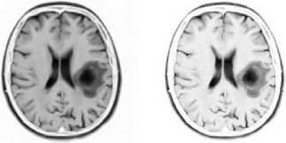
Fig.4. The images in (a) and in (b) were calculated with the ‘a’ constant set to the value of -3.0, and the ‘b’ constant set to the value of -5.0. The images in (c) and in (d) were calculated with the ‘a’ constant set to the value of -4.0, and the ‘b’ constant set to the value of -6.0. In (a) and in (c) are shown the classic-curvature images calculated from the image seen in Fig. 2a, and in (b) and in (d) are shown the intensity-curvature term before interpolation image calculated from the image seen in Fig. 2a. The circular zone surrounding the tumor inner metastasis (which is shown in dark color) is visible in bright color both in the classiccurvature images (a), (c), and in the intensity-curvature term before interpolation images (b), (d); however is more visible in (b) and in (d).

(a)                          (b)

(a)                             (b)

(c)                              (d)

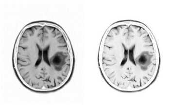
Fig.5. The images in (a) and in (b) were calculated with the ‘a’ constant set to the value of -4.0, and the ‘b’ constant set to the value of -8.0. The images in (c) and in (d) were calculated with the ‘a’ constant set to the value of 4.0, and the ‘b’ constant set to the value of 8.0. In (a) and in (c) are shown the classic-curvature images calculated from the image seen in Fig. 2a, and in (b) and in (d) are shown the intensity-curvature term before interpolation image calculated from the image seen in Fig. 2a.

The circular zone surrounding the tumor inner metastasis (which is shown in white color) is visible in gray color both in the classiccurvature images (a), (c), and in the intensity-curvature term before interpolation images (b), (d). In (a) and in (b), the circular zone is brighter than the inner metastasis, and in (c) and in (d) the circular zone is darker than the inner metastasis.

(a)

(b)

(c)

(d)

Fig.6. The images in (a) and in (b) were calculated with the ‘a’ constant set to the value of 3.0, and the ‘b’ constant set to the value of 7.0. The images in (c) and in (d) were calculated with the ‘a’ constant set to the value of 2.0, and the ‘b’ constant set to the value of 6.0. In (a) and in (c) are shown the classic-curvature images calculated from the image seen in Fig. 2a, and in (b) and in (d) are shown the intensity-curvature term before interpolation image calculated from the image seen in Fig. 2a.

The circular zone surrounding the tumor inner metastasis (which is shown in white color) is most visible in gray color in (b) than in (a), (c) and in (d).

Fig. 3, Fig. 4, Fig. 5, Fig. 6 and Fig. 7 show the classiccurvature and the intensity-curvature term before interpolation images calculated from the MRI shown in Fig. 2. The meaning of the images shown in Fig. 3, Fig. 4 and Figs. 5a and 5b is to: (i) stretch the grayscale of the MRI, and this effect is clearly visible in the classiccurvature images; and (ii) to high-define the details of the tumor region, specifically, the circular region of the tumor enclosing the inner metastasis; and this effect is clearly visible in the intensity-curvature term before interpolation images. Thus, there is difference between the grayscale of the classic-curvature images and the intensity-curvature term before interpolation images.

The circular zone surrounding the tumor inner metastasis is clearly defined in the intensity-curvature term before interpolation images, as visible in Fig. 3, Fig. 4 and Figs. 5a and 5b. To observe the aforementioned effect of high-definition, look at the darkest region of the tumor, which is circular in its essence and nature, and see how such dark region is surrounded by a brighter circular zone, which circles and surrounds it (for instance, compare Fig. 2b versus Figs. 3b, 3d) .

(a)                             (b)

(c)

Fig.7. The images in (a) and in (b) were calculated with the ‘a’ constant set to the value of 3.0, and the ‘b’ constant set to the value of 5.0. The images in (c) and in (d) were calculated with the ‘a’ constant set to the value of 2.0, and the ‘b’ constant set to the value of 5.0. In (a) and in (c) are shown the classic-curvature images calculated from the image seen in Fig. 2a, and in (b) and in (d) are shown the intensity-curvature term before interpolation image calculated from the image seen in Fig. 2a.

The circular zone surrounding the tumor inner metastasis (which is shown in white color) is most visible in gray color in (b) and in (d) than in (a) and in (d).

(d)

In Figs. 5, 6 and 7 the effect of the numerical value of the ‘a’ constant and the ‘b’ constant (for instance, in (c) and in (d) of Fig. 5 the images were calculated with the ‘a’ constant set to the value of 4.0, and the ‘b’ constant set to the value of 8.0) allows another observation on the basis of the classic-curvature image and the intensity-curvature term before interpolation image. The appearance of the images is determined by the positive values assigned to the two aforementioned constants. The classic-curvature images are smoother than the MRI shown in Fig. 2a and the intensity-curvature term before interpolation images are darker than the MRI shown in Fig. 2a. The intensitycurvature term before interpolation image shows the same behavior that was described earlier in Fig. 3, Fig. 4 and Figs. 5a and 5b, which is to circle the inner metastasis of the tumor with a gray circular zone surrounding the center of the tumor region.

The findings of this research are related to: (i) the behavior of the classic-curvature image which appears either with stretched gray scale, or smoother, respect to the MRI of Fig. 2a; and (ii) the behavior of the intensitycurvature term before interpolation image which high-defines the circular zone surrounding the tumor inner metastasis located at the center of the tumor mass . When the classic-curvature displays the stretched gray scale, the fine tuning of the brain structures can be observed with increased visibility. In general, though, the most important finding is the behavior of both the classiccurvature and the intensity-curvature term before interpolation images which determines an image with medical information related to the tumor.

• IV.    Discussion

To discuss the works herein presented, this section of the paper opens up recalling what are the technological and the theoretical requirements necessary in order to develop and bring to completion the research here conducted and/or similar research that can be undertaken when studying polynomial model functions different from the one studied in this paper. Knowledge of calculus is a necessity because of the calculation of the first and second order partial derivatives of the model function which are essential to the extent of calculating the classiccurvature. Calculus is also necessary in order to solve the integral which yields to the mathematical formulation of the intensity-curvature term before interpolation. Moreover, programming skills are required in order to implement in software the formulae of the classiccurvature and the intensity-curvature term before interpolation. Additional remarks are due so to recall that the results can be replicated because of the rigor enforced by the theoretical background of this research which is, as previously mentioned, strictly based on mathematics.

• A.    The Technological Efforts of the Research

This paper uses C++ as programming language and Visual Studio IDE as programming environment. After testing and debugging the program in Visual Studio, it is then possible to run the program with the windows command prompt and with the necessary variables as input. After the calculation of the images, the ImageJ application is used for visualization. An in depth knowledge of calculus with specific focus on the calculation of the derivatives of the model function, and the solution of the integral is required to achieve the results (see the formulae reported in the theory and methods section). A careful and further cross checking of the code was done before implementing the formulae in Visual Studio IDE since the aforementioned task is paramount to the success of the project. The program must also be tested and checked several times for correctness in order to arrive at its success. Finally, with the use of both the command prompt and ImageJ, the resulting intensity-curvature measurement approaches images were obtained and visualized. The command prompt is the integrated development environment used to run the computer program called ‘templateCurvature’ so to process the brain image. As the reader may recall from steps 8 and 9 of the theory and methods section, the process of visualization is implemented by importing the raw images which were 64 bits real image type and using the correct width and height of the image (number of pixels along the X and Y direction). Thus, for this project, the offset to the first image must always be set to 0 bytes, the number of images must be set to 1, and the gap between the images must be set to 0 bytes and also the user must check the ‘Little-Endian Byte Order’ check box since the project was developed in Intel ® environments, and finally, uncheck the remaining three check boxes, and click OK for the images to show up.

• B.    The Theoretical Efforts of the Research

This paper is concerned with the calculation of the classic-curvature and the intensity-curvature term before interpolation. The mathematical procedure outlined in this paper requires the calculation of first and second order partial derivatives of the bivariate polynomial model function fitted to the MRI data. There are two constraints that need to be satisfied by the math form of the model function. One constraint is the property of second order differentiability, which means that the model function must be such that there exists non-null (different from zero) and continuous second order partial derivatives. The second constraint is the property of the intensity-curvature term before interpolation to be nonnull when calculated at the origin of the pixel coordinate system (x, y) = (0, 0), which practically means that at least one of the second order partial derivatives calculated at (x, y) = (0, 0) must be different from zero (see yc (0, 0) in (10) in the theory and methods section).

This paper departs from a bivariate model function fitted to MRI data of the human brain in pathological state (tumor) and the mathematical procedure developed herein consists of two steps [7, 12-17]:

• 1.    The calculation of the classic-curvature.

• 2.    The calculation of the intensity-curvature term before interpolation.

The classic-curvature and the intensity-curvature term before interpolation are termed as intensity-curvature measurement approaches [7]. Fitting the model function to the MRI data allows the development of the mathematical procedure and thus the calculation of the two intensity-curvature measurement approaches (which are images). The model function is the driving force at the basis of the mathematical procedure. The intensitycurvature measurement approaches images are calculated from the collected MRI image when the model function is implemented. Consequentially, the appearance of the resulting intensity-curvature measurement approaches strictly depends on the model function fitted to the MRI image data.

• V.    Conclusion

This research studies the behavior of two intensitycurvature measurement approaches which are called classic-curvature and intensity-curvature term before interpolation. The two intensity-curvature measurement approaches consist of mathematical methodology that can be used to post-process Magnetic Resonance Imaging (MRI) of the human brain. The study is undertaken fitting a bivariate polynomial model function and postprocessing a two-dimensional MRI image. The full mathematical procedure for the calculation of the two intensity-curvature measurement approaches is reported. The model function is parametric in two constants and so allows obtaining intensity-curvature measurement approaches with diverse appearance. The technical details of the procedure used to run the computer program that implements the mathematical procedure were described. Also, the details relevant to the visualization of the resulting images are provided. The classic-curvature images reveals the characteristic of smoothing the original MRI image. The analysis also reveals the capability of the intensity-curvature term before interpolation images to high-define the tumor structures which are seen in the MRI. Therefore for the first time in the literature this paper reports on the novelty of the characterization of the intensity-curvature term before interpolation. The significance of the aforementioned novelty relates to an in depth and further study of the medical intensity-curvature map of the human brain structures [7].

Acknowledgment

The author is grateful to Assistant Professor Carlo Ciulla for his patience, encouragement and kindness, which brought this work to completion. The author is also grateful to Dr. Dimitar Veljanovski, and Dr. Filip A. Risteski at the General Hospital 8-mi Septemvri, Department of Radiology, Boulevard 8th September, 1000, Skopje, Macedonia, because of the MRI image provided for these studies. The MRI scanning procedures were conducted in compliance with the ethical standards set by the General Hospital 8-mi Septemvri, Skopje, Macedonia. Last but not least, the author is sincerely grateful to Pastor Pal Katona and Mrs. Ibolya Katona whom supported me in diverse ways.