Child based Level-Wise List Scheduling Algorithm

Cloud computing fulfill the demand of resources through internet with the help of virtualization. There are three main entities: cloud users, service providers and cloud services. Cloud service provider provides common resources and services on demand to cloud users. Services will be chargeable by the Service provider; customer pays for what a customer used. There are different types of services including operating systems, storage space, and environment for application development and processing capabilities[1]. According to the business requirements, customer can increase or decrease the resource usage. Cloud provide flexibility to the customer, they can access resources on different devices such as laptops, personal devices, smart phones

• & tablets. It has the minimum chances of infrastructure failure.

Broadly cloud computing environments are of 3 types. Private clouds (internal cloud): Exists privately in an organization and facilitates special benefits.

Public clouds – It is for public use. Some organizations managed and offered services to customers. Highly scalable and reliable but less secure.

Hybrid clouds - it is the mixture of the both environments mentioned above^[2].

Cloud services accessed through Application Programming Interfaces (APIs). The characteristics of cloud environment are Multi-sharing, Scalability, Availability and Reliability.

Cloud environment provides services broadly categorized as follows:

IaaS ( Infrastructure as a Service ) - User can access only the resources required without knowledge of any other details like Elastic Computing Cloud of Amazon and Amazon’s Storage Service facilitate flexible computing capacity (CPU cycles)^[3] and rental base retrieving or managing large quantity of data anywhere anytime from internet respectively^[4].

PaaS ( Platform as a Service ) - it gives different environments for development of specific application. Like Google App Engine which take care of the application's execution developed on engine^[5].

SaaS ( Software as a Service ) – no development, no maintenance at user end. Application or software facilitate by the provider on internet like MS-Dynamics a CRM tool provided by Microsoft managed customer’s information online^[6].

In the paper, a task scheduling algorithm which used the principle of list scheduling technique has been proposed named Child Based Level-Wise List Scheduling (CBLWLS) algorithm, which effectively schedules the tasks with the help of priority on to the processors.

Other parts of the paper are: problem description explained in Section II. Section III explained our proposed workflow scheduling algorithm. Section IV shows a sample execution. Experimental details and simulation results are shown in Section V. Conclusion with future scope in Section VI.

• II.    Problem Description

Cloud applications are modeled into workflows. Workflow applications are executed in a particular order because they have group of different tasks which achieves a particular result called task scheduling. To achieve efficient task scheduling we use task scheduling algorithms. Main goal of these algorithms are to assign the tasks to the available processors and generate minimum completion time called makespan.

Scheduling of workflow is most important factor to fulfill the requirement of cloud user as well as cloud provider. Efficient scheduling of workflow is necessary to reduce overall execution time and cost incurred to complete the workflow execution [7].

Generally, two types of task scheduling algorithms are there: Static has information like estimation time of job execution, structure, data dependencies, resource mapping and amount of data to be transferred before execution and takes decisions at compile time. Dynamic algorithm estimates the information before execution at the ready state of job and decisions made at run time.

Good scheduling quality and performance are provided by algorithms based on the list scheduling. In these, a priority list is generated from given graph. Based on priority, tasks are picked up and allocated to that processors who gives minimum execution time. Like heterogeneous earliest finish time algorithm (HEFT) [8].

Directed acyclic graph (DAG) represents a workflow and denoted by G ( v, e ). Where, v denotes quantity of nodes and data dependency between tasks denoted by e ^[9]. Fig. 1, shows a sample workflow graph G with the dependencies among different tasks.

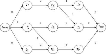
Fig.1. Sample DAG [10]

In Fig. 1, task t_entry acts as entry task which has no parent and task t_exit act as an exit task with no child node. The child tasks t₁ , t₂ and t₃ are executed after parent task t entry . Parent task gives input to child tasks. After the completion of tasks t 7 , t 8 and t 9 , task t exit is executed. Each node is assigned estimated computation time and each edge represent estimated communication time.

There is requirement of task scheduling algorithms that in a task graph, there should be exactly one exit and exactly one entry task. If there are multiple exit or entry tasks then always add dummy task at the end and in the beginning of the workflow, respectively. Assign zero execution time to the dummy tasks and connect to exit and entry tasks with zero-weight dependencies. When values of nodes and edges are calculated for a DAG with different methods then there is a considerable effect on schedule [11].

The goal of the algorithm is to provide better quality of schedule (or output with minimum schedule length). To achieve efficient scheduling, a list scheduling algorithm has been implemented considering time and cost factor. Time factor considers execution time and communication time. Cost factor consider cost incurred to running the tasks on processors. It applies general approach, give priority to tasks in workflow then according to priority the tasks are allocated to the optimal resource.

• III.    Proposed cblwls scheduling algorithm

Child Based Level-Wise List Scheduling (CBLWLS) algorithm is a type of list heuristic scheduling which prioritizes and schedules workflow tasks on processors according to their priorities. This algorithm consists three phases which are explained as follows:

• a)    Level Sorting Phase: In a given DAG add dummy entry or exit task if required then traverse it from up to down at every level for grouping independent tasks. So that same level tasks can be submit for parallel execution. Entry tasks at Level 0. If level i contains all tasks v k and all edges ( v j , v k ) then there exists at least one edge ( v j , v k ) from level i-1 to i and tasks v j is in a level less than i . Exit task in the last level ^[12].

• b)    Task Prioritization Phase: In this phase, calculate rank and assigned to each task with the help of attributes Data Received Time ( DRT ) from parent, Average Computation Time of Node ( ACTN ), Data Transfer Time ( DTT ) to child and Average Computation Time of Child ( ACTC ). These

attributes are explained as follows:

• 1.    Data Received Time (DRT):  It is the

• 2.    Average Computation Time of Node (ACTN): It is the average of computation time of a task n i on all processors p ^[13].

• 3.    Data Transfer Time (DTT):  It is the

• 4.    Average Computation Time of a Child (ACTC): The ACTC of a task n i is the average computation time of a child on all the processors p .

• 5.    Give highest priority to the task with highest rank value at each level followed by task with next highest rank and so on. In case of tie high priority assign to the task having higher ACTN value.

communication time of a task n i to transfer the data from immediate parent task to task n i ; for an entry node DRT ( n entry ) =0.

communication time of a task n_i to transfer the data from task n_i to its immediate successor task; for an exit node DTT ( n exit )= 0.

The rank of each task n i is calculated with DRT, ACTN, DTT and ACTC values and is given by:

Rank (n_i) =max (DRT (n_i)) + ACTN (n_i) + max(DTT(n i , child x)+ACTC(child x))

Where n represent a node of workflow, i represent its number and x represents child of node n .

• c)    Processor Allocation Phase: At each level, highest rank value task is selected. Calculate EST (Earliest Start Time) and EFT (Earliest Finish Time) value for selected task on every processor. Task is assigned to the processor who gives minimum EFT .

• IV.    Sample Workflow

Fig. 2, shows sample workflow^[14] with all its dependencies and communication time and Table 1, shows computation time of the tasks on individual processor and the average computation time of node ( ACTN(n i ) ). Here entry task is T 0 and exit task is T 9 .

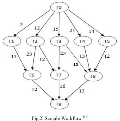
Table 1. Computation time in seconds for sample workflow [14]

Task	P 0	P 1	P 2	ACTN(n i )
T 0	9	14	16	13
T 1	13	18	19	16
T 2	11	13	19	14
T 3	8	13	17	12
T 4	10	12	13	11
T 5	9	13	16	12
T 6	7	11	15	11
T 7	5	11	14	10
T 8	12	18	20	16
T 9	7	10	21	12

Phase wise solution of sample workflow using CBLWLS is as follows:

• a)    Level Sorting Phase: There are 4 levels in the DAG.

Apply algorithm to levels one by one.

Level 1 has node: T₀

Level 2 has nodes: T₁, T₂, T₃, T₄, T₅

Level 3 has nodes: T 6 , T 7 , T 8

Level 4 has node: T 9

• b)    Task Prioritization Phase:

For level 1: there is only node T 0 .

Rank (T0) = max (DRT (T0)) + ACTN (T0) + max (DTT (T0, child x) +ACTC (child x))

DRT (T 0 ) =0; ACTN (T 0 ) =13;

For children’s of T 0 ,

Calculate (DTT (T 0 , child x) +ACTC (child x)

For T 1 = DTT (T 0 , T 1 ) + ACTC (T 1 ) =5+16=21

For T 2 = DTT (T 0 , T 2 ) + ACTC (T 2 ) =12+14=26

For T 3 = DTT (T 0 , T 3 ) + ACTC (T 3 ) =15+12=27

For T 4 = DTT (T 0 , T 4 ) + ACTC (T 0 ) =21+11=32

For T 5 = DTT (T 0 , T 5 ) + ACTC (T 0 ) =14+12=26

Maximum value 32 is selected.

Rank ( T 0 ) = 0 + 13 + 32=45.

Arrange level 1 nodes in descending order of rank. So nodes will be executed in order T 0 .

Table 2, shows level, calculated value of DRT, ACTN, max(DTT+ACTC) , rank of each node and priority of node within its level.

Table 2. Priority computation for sample workflow

Level	Task	DRT	ACTN	max( DTT +ACTC)	Rank	Priority
1	T0	0	13	32	45	1
2	T1	5	16	26	47	5
2	T2	12	14	34	60	2
2	T3	15	12	33	60	3
2	T4	21	11	29	61	1
2	T5	14	12	28	54	4
3	T6	23	11	24	58	2
3	T7	23	10	28	61	1
3	T8	13	16	25	54	3
4	T9	16	12	0	28	1

So the tasks execution order is T 0 , T 4 , T 2 , T 3 , T 5 , T 1 , T 7 , T 6 , T 8 , T 9 .

• c)    Processor Allocation Phase

Assign the tasks to processor having minimum EFT . Table 3, shows EST and EFT of selected task on each processor. The bold values indicate that the T_i task allocated to P_p processor.

Makespan by Child Based Level-Wise List Scheduling Algorithm is 76 seconds.

The generated schedule length of CBLWLS algorithm is shown in Fig. 3.

Table 3. Processor Allocation for Sample Workflow

	Processor P 0		Processor P 1		Processor P 2
Tasks	EST	EFT	EST	EFT	EST	EFT
T 0	0	9	0	14	0	16
T 4	9	19	30	42	30	43
T 2	19	30	21	34	21	40
T 3	30	38	24	37	24	41
T 5	30	39	37	50	23	39
T 1	39	52	37	55	14	33
T 7	60	65	42	53	60	74
T 6	48	55	53	64	53	68
T 8	55	67	53	71	51	71
T 9	69	76	80	90	80	101

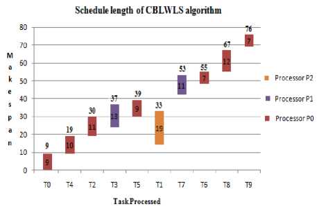
Fig.3. Schedule Length by CBLWLS

The comparison of schedule length (makespan) of CBLWLS and HEFT is shown in Fig. 4. The makespan by CBLWLS algorithm is 76, which is shorter than the makespan obtained by HEFT algorithm which is 81. It is observed that the proposed CBLWLS algorithm is producing better schedule length as compared to HEFT algorithm.

Makespan

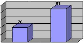
CBLWLS

HEFT

Fig.4. Makespan comparison of CBLWLS and HEFT

Epigenomics: It was developed by Pegasus Team and USC Epigenome Center. It is used for the automation of different operations in genome sequence processing.

Fig. 5, shows its structure.

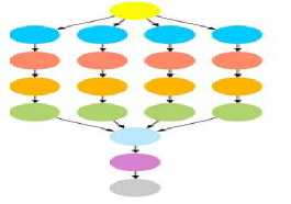
Fig.5. Epigenomics Structure [16]

This workflow is available in DAX (Directed Acyclic Graph in XML) format and used as input. The two algorithms CBLWLS and HEFT are implemented using JAVA on Intel B960 Dual Core Processor machine with HDD of 500 GB and RAM of 2 GB having Windows 7 OS using Eclipse. The computation time in second of a particular node on processor, input and output communication data of a node in MB and relationship between the nodes are fetched from the DAX. By assuming network bandwidth 1MB/s converted communication data into communication time. Example: 50 MB data required 50 seconds to transfer data. To simulate a cloud environment, parameters as shown in Table 4 are defined.

Table 4. Parameter Settings for Cloud Environment

Parameter	Value
Number of Processors	10-25
Number of Workflows	4
Tasks per Workflow	25-1000

Processor will execute the tasks in cycles. We assume that 1 cycle of 30 second. Now we will calculate number of cycles for cost calculation as follows:

If execution time divided by 30 is equal to zero, then

Number of cycle = execution time/30;

Otherwise

Number of cycle = (execution time/30) +1;

The processors are different in speed and cost of execution. So fastest processor takes less time but high cost as compared to slowest processor who takes more time but less cost for the same task. Table 5 shows the assumption of execution time and cost of execution of tasks on the processor P_i where i is the number of processor.

Table 5. Processor execution time and Cost of execution

• V.    Experimental Detail and Simulation Results

The effectiveness of proposed algorithm is proved theoretically for sample graph and experimentally for Epigenomics workflow structure used in different scientific applications[15].

Processor Type	Execution Time	Cost of Execution
Fastest Processor ( P 0 )	(Fetched from DAX*100)	300 units per cycle
Other Processor ( P i )	P 0 +((P 0 *i* 10/)100))	(300-( i *10)) units per cycle

• A)    Comparison Metrics

The following metrics have been taken to evaluate the proposed algorithm.

Makespan: It is total length of the schedule (that is, when all the jobs have finished). The algorithm that generates less makespan is efficient algorithm.

Cost: It is the total cost occurred to run the different tasks on different processors. Efficient algorithm minimizes the cost of execution.

SLR: it is the ratio of actual makespan to the makespan obtained when all the tasks assigned to fastest processor, so that is no communication time involved. An algorithm having smaller SLR value is a more efficient algorithm. It is calculated by following equation:

SLR =

actual makespan

/      makespan obtained

/ when all tasks on fastest processor

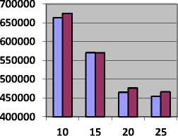
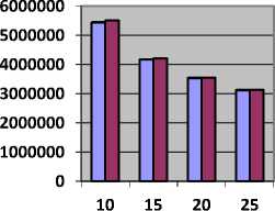
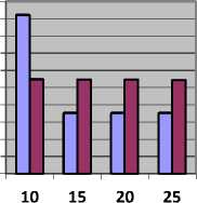
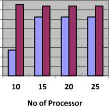
• 1)    Makespan

All the graphs drawn with the variation of no of processors and nodes in a workflow in the Epigenomics model. In graphs x-axis represents number of processors.

Table 6 shows the value of makespan and Fig. 6, represents makespan in seconds obtained with CBLWSL and HEFT with y-axis represents makespan in seconds.

Table 6. Makespan value in second for Epigenomics Model

No of Nodes No of Processors		25	50	100	1000
10	CBLWLS	57403	71880	663774	5441132
	HEFT	60121	81913	675074	5500792
15	CBLWLS	57403	79180	571071	4174570
	HEFT	60121	81583	570642	4206692
20	CBLWLS	57403	79180	465310	3537894
	HEFT	60121	81583	476692	3545463
25	CBLWLS	57403	79180	454648	3120739
	HEFT	60121	81583	466451	3130790

• B)    Comparative Analysis of Workflows from scientific application

  No of Nodes 25

  
  

No of Nodes 100

О

CBLWLS

HEFT

No of Processor

о

CBLWLS

HEFT

No of Processor

No of Nodes 50

No of Nodes 1000

CBLWLS

HEFT

No of Processor

CBLWLS

HEFT

No of Processor

Fig.6. Makespan for Epigenomics Model

As shown in Table 6 and Fig. 6, in most of the cases makespan obtained by CBLWSL is less than HEFT. In graphs, makespan decreases as number of processors increases because tasks have more tendency to get execute in parallel. In term of percentage CBLWLS decrease the makespan by 0.896 % then HEFT. So CBLWSL is more efficient.

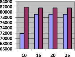
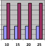
• 2)    Cost

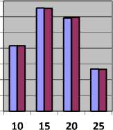
Table 7, shows the value of cost and Fig. 7, represents cost in units obtained by CBLWSL and HEFT with y-axis represents cost.

Table 7. Cost in units for Epigenomics Model

No of Nodes No of Processors		25	50	100	1000
10	CBLWLS	1936140	4860430	47561050	455734730
	HEFT	1937080	4852960	47545230	455802540
15	CBLWLS	1936140	4849060	48481310	467719860
	HEFT	1937080	4852940	48477290	467663250
20	CBLWLS	1936140	4849060	48277760	464635910
	HEFT	1937080	4852940	48259570	464755770
25	CBLWLS	1936140	4849060	47651490	448410520
	HEFT	1937080	4852880	47631640	448327360

As shown in Table 7 and Fig. 7, in most of the cases cost obtained by CBLWSL is less than or nearly equal to the cost obtained by HEFT. So the CBLWSL maintained the cost of execution rather than increasing the cost. We can’t generalize the pattern obtained in graphs for cost incurred because calculation of cost depends on processor cycle and computation time of task. In term of percentage CBLWLS increase the cost by 0.000018 % then HEFT which is very less than makespan.

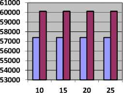
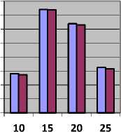
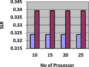
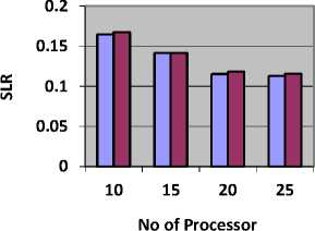
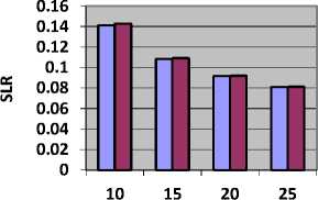
• 3)    SLR

Table 8 shows the value of SLR and Fig. 8, represents SLR obtained by CBLWSL and HEFT with y-axis represents SLR.

Table 8. SLR value for Epigenomics Model

No of Nodes No of Processors		25	50	100	1000
10	CBLWLS	0.323959	0.173625	0.164546	0.141154
	HEFT	0.339298	0.197859	0.167347	0.142702
15	CBLWLS	0.323959	0.191258	0.141565	0.108297
	HEFT	0.339298	0.197062	0.141459	0.109130
20	CBLWLS	0.323959	0.191258	0.115348	0.091780
	HEFT	0.339298	0.197062	0.118169	0.091976
25	CBLWLS	0.323959	0.191258	0.112705	0.080958
	HEFT	0.339298	0.197062	0.115631	0.081219

No of Nodes 25

No of Nodes 100

□ CBLWLS

□ HEFT

No of Processor

□ CBLWLS о HEFT

No of Processor

No of Nodes 50

No of Nodes 1000

□ CBLWLS о HEFT

No of Processor

□ CBLWLS о HEFT

No of Processor

Fig.7. Cost for Epigenomics Model

No of Nodes 25

No of Nodes 100

□ CBLWLS о HEFT

□ CBLWLS

□ HEFT

No of Nodes 50

No of Nodes 1000

0.2 0.195 0.19 0.185 s   .0.18

0.175

0.17 0.165

0.16

□ CBLWLS

□ HEFT

□ CBLWLS о HEFT

No of Processor

Fig.8. SLR for Epigenomics Model

As shown in Table 8 and Fig. 8, in most of the cases SLR obtained by CBLWSL is less than the HEFT. So the CBLWSL is more efficient algorithm. In graphs, SLR decreases as number of processors increases because tasks have more tendency to get execute in parallel and gives less makespan which results in low SLR.

• VI. Conclusion and Future Scope

  In this paper, Child Based Level-Wise List Scheduling (CBLWLS) algorithm is proposed, which is a non-preemptive static type of scheduling algorithm for heterogeneous computing environment. The CBLWLS algorithm is evaluated on Epigenomics model. The performance of the algorithm is compared with HEFT algorithm based on the execution time, cost incurred and SLR. The effect of variation of number of machines and number of tasks on makespan, cost and SLR has been studied. It has been found that if we take the average of result and calculate the percentage then CBLWLS Algorithm decrease the makespan by 0.896 % but increase the cost by 0.000018% than HEFT which is very less than makespan. So CBLWLS performed better than HEFT on all the parameters.

For future work, the same priority techniques may be tested on LIGO Inspiral Analysis and Montage model, may be using time deadline and cost constraints. Various other QoS parameters such as reliability and fault tolerance may be applied. The work of paper may be applied in real world cloud computation systems for scheduling purposes.