Classification of agricultural crops from middle-resolution satellite images using Gaussian processes based method

Remote sensing is a useful tool for agricultural management and decision making [1]. The vast diversity of available instruments makes possible the effective and low-cost observations of agricultural lands condition [2]. The use of remote sensing data for agricultural land monitoring enables to control arable land areas and various types of cultures growing there. Particularly, with the use of satellite data collected over different time periods, it is possible to track changes in the state of vegetation and to assess the plant growth rate and type [2-4].

An important problem arising during analysis of the satellite images is objects recognition. There are several methods of image classification for agricultural land analysis [3]. The most widely used methods for classifying crop species from satellite images are maximum likelihood classifier (MLC) and support vector machine (SVM). MLC is a simple parametric classifier [5], while nonparametric SVM use optimization algorithms to determine the optimal boundaries between classes [6]. These methods demonstrate quite good results. For example, in the work of Devadas et al., 2012, the accuracy of classifying several classes of cultures (fallow, crop, pasture, woody) using Landsat satellite data is 93% with MLC methods and 78% with SVM methods [7]. However, the accuracy of these methods is not always satisfactory for specific applications and images. In the work of Topalogu et al., 2016, the accuracy of classifying a general class of cultures using Landsat satellite data is about 45.45% with MLC and 77.42% with SVM methods [8]. In the work of Waske, 2007, the accuracy of classifying several classes (arable crops, cereal, canola, root crops, grassland, orchard, – 910 – forest, urban) using Landsat satellite data is about 62% with MLC methods and 64% with SVM methods [9].

The aim of this work is to implement the classical GP based techniques on multi-temporal images of arable land areas acquired by the Landsat satellite in order to classify species of agriculture plants grown in selected areas of Krasnoyarsk Krai (Russia).

Remote sensing data and the study area

Middle-resolution satellite imagers are best suited for studying local test areas by using multitemporal images. In this paper we employed imagery of the Landsat 8 satellite (American Earth observation satellite launched on 11 February 2013), which allows obtaining up to 400 scenes every day. This satellite acquires images in 11 spectral channels by using Operational Land Imager (OLI) and Thermal Infrared Sensor (TIRS) instruments. OLI operates in 9 spectral channels while TIRS forms images in channels 10 and 11 [10]. Landsat 8 level 1products used were derived from the open source of United States Geological Survey (USGS).

Level 1 images are represented in the form of 16-bit digital numbers which can be transformed to the TOA spectral radiance

L ( X ) = M l ( X ) D n + A l ( X ) ,                                       (1)

where AL и ML are – additive and multiplicative parameters or to the TOA spectral reflectance p (X ) = Mp (X )Dn + A (X )

sinθ

SE where θSE is the solar elevation angle. The calibration parameters can be obtained from metadata.

The training data were obtained from images with 8071 × 8161 pixel resolution. We employed the spectral channels of visible and near-infrared spectral region for the formation of the additive color model (RGB) and calculating vegetation indexes. The image data were acquired from the Georeferencing Tagged Image File Format GEOTIFF with Universal Transverse Mercator (UTM) projection in coordinate World Geodetic System (WGS).

To increase the accuracy of the analysis, we have used cloudless and terrain-corrected images for years 2015 and 2016 acquired during the period of active plant growth. The available georeferencing information allowed us to cut automatically the training data from the coordinated plot of 219 × 196 pixels (about 16 km2).

The ground-based information is available for agricultural fields of Suhobuzimsky district, located in the central part of Krasnoyarsk Krai, Russia with a total area of 5612 km2. The fields of JSC Uchkhoz “Minderlinskoe” are labeled as containing different crops (wheat, oats and barley), annual and perennial grasses or as a fallow (Fig. 1).

The test data were obtained from the same satellite imagery that were used for the training set in years 2015-2016 but acquired from a different area. The test sites are from Plemzavod territory of JSC “Taiga” Suhobuzimsky area of 546 × 627 pixels, which corresponds to the area on the Earth’s surface of 135 km2. The test fields are also labeled as wheat, oats, barley, annual grasses, perennial grasses and fallow (Fig. 2).

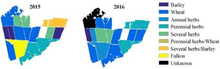
Fig. 1. Maps of agriculture fields of JSC Uchkhoz “Minderlinskoe” for years 2015-2016

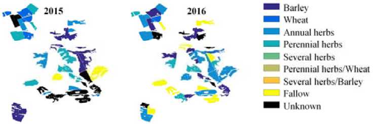
Fig. 2. Maps of agriculture fields of Plemzavod territory of JSC “Taiga” for years 2014-2015

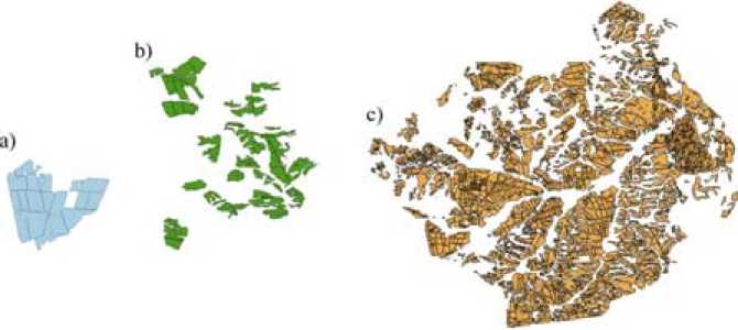
Fig. 3. Mask of the fields of Suhobuzimsky district, where (a) is the training land of JSC Uchkhoz “Minderlin-skoe”, (b) is the test land of JSC Plemzavod “Taiga”, (c) shows the total sown area of the region, which includes the areas shown in (a) and (b)

The verification was performed using field data presented at the geoinformation portal of the Institute of Space and Information Technologies, Siberian Federal University [11].

Pre-processing of the satellite data was performed using the software ENVI 5.2 and a geographic information system QGIS 2.8.2. This procedure consisted of several stages: (i) combining spectral channels from 2 to 5 for all satellite images, (ii) creating a mask for input and test plots on the vegetation field map (Fig. 3), (iii) cropping satellite images according to the – 912 –

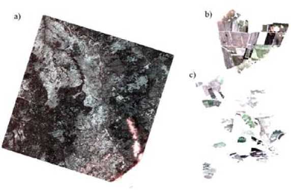
Fig. 4. Satellite image with the capture of fields of Suhobuzimsky district for 16.05.2016, where (а) is the original image, (b) is the training land of JSC Uchkhoz “Minderlinskoe”, (с) is the test land of JSC Plemzavod “Taiga”

previously created masks (as an example, see image for 16.05.2016 on Fig. 4), (iv) saving images in the format GEOTIFF.

Data analysis and pre-processing

In the pre-processing stage, 21 multitemporal satellite images were prepared, of which 12 images were the training data (6 for 2015, 6 for 2016), and 9 images were the test data (5 for 2015, 4 for 2016). Table 1 shows the total number of fields and pixels for each culture for a training and test set in two years.

Table 1 shows that the number of test samples is much higher than the number of training samples. The main reason for choosing the fields of JSC Uchkhoz “Minderlinskoe” as the training set was the greater amount of data for the whole period of the crop life cycle, in contrast to the fields of JSC Plemzavod “Taiga”.

Table 1. Total number of fields and pixels per culture

Culture	Training dataset				Test dataset
	2015		2016		2015		2016
	Number of fields	Number оf pixels	Number of fields	Number оf pixels	Number of fields	Number оf pixels	Number of fields	Number оf pixels
Barley	3	2386	1	996	16	14079	11	7940
Wheat	6	7158	7	9245	8	6016	4	4032
Annual herbs	2	4227	2	2805	12	11812	16	17960
Perennial herbs	-	-	2	4227	-	-	7	7288
Fallow	1	2241	-	-	-	-	-	-
Total	12	16012	12	17273	36	31907	38	37220

The classification algorithm is based on the use of vegetation maps, satellite imagery, and on the analysis of Normalized Difference Vegetation Index (NDVI). This indicator is widely used for data analysis and monitoring of the state of vegetation on a global and continental scale [1]. NDVI is a simple quantitative indicator of photosynthetic active biomass, often referred to as the vegetation index. NDVI is calculated according to the data of broad spectral zones as follows

NDVI = ^{P nir P red} , ^P NIR + ^P RED

where, ρ_NIR is the reflection coefficient in the near infrared, and ρ_RED is the reflection coefficient in the red region of the spectrum. The absolute values of vegetation index range from -1 to +1. For vegetation, NDVI takes positive values from 0.2 to 0.9 on average. Therefore, the greener the vegetation represented by multispectral images, the closer the NDVI index is to 1.

Time dependences of NDVI values for different cultures were calculated as follows: NDVI was calculated per pixel and then the values obtained were averaged over each field and the corresponding culture on the image. The averaged NDVI values of the training and test sets are shown in Fig. 5. The error bars on the plots show the 95% range of NDVI values that includes all values from 2.5 up to 97.5 percentage points.

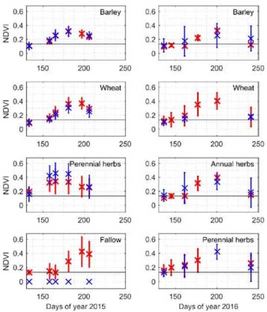
Fig. 5. The NDVI of vegetation plotted against days of year 2015 and 2016, where the training set is represented by red crosses, the test set is shown by blue crosses, and the black horizontal line is the boundary of the soil. The error bars show the 95% range of NDVI values

The boundary of the soil shown in Fig. 5 by the black horizontal line was determined from the imagery of fields with fallow acquired during the spring period. This boundary allows us to distinguish clearly the average NDVI of vegetation from the NDVI of the open soil. It should also be noted that usually, the NDVI index value close to 0.6 (for Landsat images) corresponds to the area with a dense vegetation cover, while the value of about 0.3 are characteristic for the areas with mixed cover, i.e. immature vegetation or crops at the end of their life cycle [1].

NDVI time-series modeling

To solve the problem of vegetation recognition on satellite images, we have proposed a method which can be employed also for predicting the crops found in the surrounding areas. The method consists of two stages: regression and classification. The aim of the first stage consists in NDVI timeseries modeling by using the Gaussian Process Regression (GPR) [12-14]. We are interested in predicting the NDVI values for the whole active season day by day, so that we can later use this information for the final classification step.

Let us consider a problem y = f(t) + ε,                                                                           (4)

where t is an input variable (the time point in our case), y is a scalar response (NDVI value), f is some 2

model function, considered as a random process, and e ~ N ( 0, ст ) is a model error, considered as the normally distributed random noise with zero expectation and the variance σ 2 .

Let f is Gaussian process (GP). Then for any finite set of inputs T = {t 1 ,..., t N }, the corresponding set of random function variables F = { fo., ^fN ^} has a joint Gaussian dtit-Mun

, p ( F,T )         )                                                          ( ⁵⁾

where K = { K i j }    is the covariance matrix constructed from the covariance function

, j

K , j . K ⁽ t i ^, t, ) = Ef ( t ) ^{f ( tj )                                                     (6)}

Let we have N measurements Y = { y , ,..., y_y У ^{in time} P ^oints T = {t i ,..., t N ^} T ^{and we need to} estimate y * in the time point t * employing the model (1). In this case, the extended random vector { y ,..., y , y } has also multidimensional normal distribution

Y

y *

~

N 0,

K

K *

^K * ^T

К

**

where K * =[ K (t*, t1),..., K (t*, tN)], K** = K (t*, t*) and I is the identity matrix of needed size. It can be shown that the conditional (posterior) distribution of y* is also Gaussian and can be expressed as

p ( y * | Y ) = N ( K * ( K + ст ² 1 Г1 Y , K ** - K * ( K + ст ² 1 Г1 K T + ст 2 ).                (8)

Then the best estimate y of y is the expectation corresponding to this distribution **

y* = K . ( K . , ² I)CT ,                                                        ⁽⁹⁾

and the uncertainty ν of this estimate is the variance v = K** - K* (K + о21)-1 K* + о2.

The estimate (9) can be easily extended to the case when f has some nonzero expectation function ^ ( t ) = Ef ( t ). In this case, the estimate can be expressed as

y * = m ( t * ) + K * ( K + о ² 1 ) ^{- 1}( Y -M ),

where

M = { ^ ( t^,..., _M ( t N )} ^r .

We used the constant expectation and the squared exponential covariance (or kernel) function

K ( t i , t j ) = h exp

—

⁽ ti ^— t j ^{) 2}

where h is the scale factor of the response and λ is the input length-scale hyperparameter, which controls the smoothness of the regression function. Such types of functions were chosen to produce the smooth regression curve, since it is obvious that NDVI variations from a day to another should be small enough. GPs also have a noise parameter. This parameter controls how tight should be the fit of the posterior function to the data points.

The unknown hyperparameters were obtained from the training set by using minimization of the negative logarithmic likelihood function. The regression results are represented in Fig. 6 for the years 2015 and 2016. Grey areas show the uncertainty of the regression. As we can see, GPR allows us to

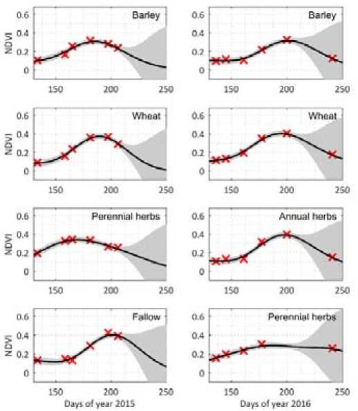
Fig. 6. Regression model of NDVI for training dataset observed in years 2015-2016

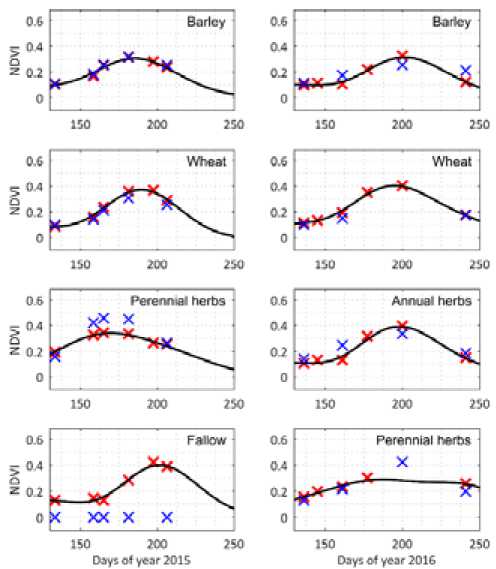
Fig. 7. Classification of average NDVI for different crops in years 2015-2016

interpolate well the NDVI values during the vegetation period. We should also notice that areas with lower density of data have greater uncertainty.

Classification method

On the next step, we employ a simple classifier whose performance should be compared with the precision of the acquired data. The temporal data from each area in a new image is compared to the learned regression model. The classifier will assign the class k , which yields the lowest mean squared error (MSE) between the test points y(t) and the regression values yˆk (t) at those temporal points for each crop/class. Formally, we have k = arg min £ (y(t) - yk(t))2 .                                                 (14)

kt

Figure 7 shows the average NDVI for the different crops in the test image of years 20152016.

Notice that the values for the test image (blue crosses) are similar to those obtained for the train image, which will result in an accurate classification. However, for year 2015 we see higher NDVI values for perennial herbs. It should be carefully investigated why this happened. The reason for this may be that this class comprises several types of crops, which could have different NDVI profiles. In addition, we notice an unseen value in 2016 for the same class, which is not close to the learned curve, indicating that the training data was insufficient.

Results and discussion

Finally, we present the results obtained for the implemented classification method. The classification of agricultural crops based on NDVI of was carried out, where the time variability of this vegetation index was obtained from satellite images of OLI Landsat 8. NDVI is the most important feature, which affects the overall accuracy of classification by Gauss method. The test image consisted of 56 regions with different crops. We selected only those which contained one of the plants plotted in Fig. 7 (Notice that we did not have training data for annual herbs in 2015, so in this case we only considered 3 classes). Fig. 8 shows a simple diagram that depicts the whole classification process.

The results of the classification are presented in Tables 2 and 3. The algorithm always distinguishes class 3 from classes 1 and 2, although these latter classes are often confused. The reason lies in the similar NDVI profile, suggesting that additional information on those areas should be used, like weather, soil and other factors that were not used in this work.

The overall accuracy is low. Only the first class obtains a decent precision. We notice that wheat is often assigned to class barley, which suggest again that additional data should be used. Additionally, NDVI average profiles for year 2016 seem to differ noticeably from the learned regression, as shown on Fig. 7. NDVI profiles should be checked individually to detect acquisition errors or cloud presence that may be worsening the performance of the algorithm. The low classification accuracy can also be addressed to the following reasons: classification errors between crops and pastures; a high amount of precipitation during the growing season, which leads to the difficulties in recognizing crops on the images; cloud cover during the summer.

For comparison, we present in Table 4 the results of classification by the simplest metric classifier based [15]. As can be seen from Table 4, the overall classification accuracy of crops by the metric

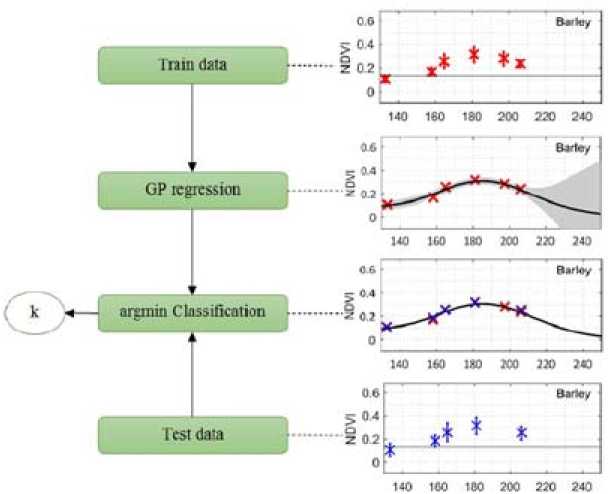
Fig. 8. The classification algorithm

Table 2. The confusion matrix and overall accuracy for year 2015 are by the Gauss method

Classes		Predicted class
		Barley	Wheat	Perennial herbs	Total
-й g "Й й Й о	Barley	12	4	0	16
	Wheat	4	4	0	8
	Perennial herbs	0	0	12	12
	Total	16	8	12	36

Overall accuracy = 77.78%

Table 3. The confusion matrix and overall accuracy for year 2016 are by the Gauss method

Classes		Predicted class
		Barley	Wheat	Annual herbs	Perennial herbs	Total
-Й й й Й о О	Barley	12	4	0	0	16
	Wheat	4	4	0	0	8
	Annual herbs	0	6	0	1	7
	Perennial herbs	0	0	0	12	12
	Total	16	14	0	13	43
Overall accuracy = 65.12%

Table 4. The confusion matrix and overall precision for year 2015 are by the metric classifier

Classes Predicted class Barley Wheat Perennial herbs Total -Й й -й й Й о Barley 7 3 0 10 Wheat 1 2 0 3 Perennial herbs 0 2 0 2 Total 8 7 0 15 Overall accuracy = 60% classifier is 60% for year 2015. For data of year 2016, the metric classifier could not classify crops presumably due to the small number of test data points.

We note that a separate analysis, carried out by combining several classes–barley and wheat–into single spring crops class showed that the overall accuracy of the Gauss method is 97.02% for year 2015 and 83.72% for year 2016.

Conclusions

In this paper, we use the Gaussian process to classify crops on Landsat satellite data imagery. The results of this study show that GР demonstrates high precision in recognizing barley and wheat crops against perennial grasses. However, there are difficulties in recognizing individual vegetation types – 919 – due to the almost identical time-series of NDVI. The overall classification accuracy of crops by the Gaussian method is 77.78% for year 2015 and 65.12% for 2016. The overall classification accuracy of crops by the metric classifier method is 60% for year 2015. Comparison of the overall accuracy of the GP classification with the results obtained by using the metric classification clearly shows the advantage of GP. Thus, the Gaussian process has perspectives in its further use for classifying objects from remote sensing data.

Acknowledgments

These results are obtained under funding support from the Russian Science Foundation (No. 1611-00007).