Classification of Brain Activity in Emotional States Using HOS Analysis

Published Online February 2012 in MECS

Emotion is a complex psycho-physiological behavioral of mind as interacting with biochemical and environmental influences. Emotion fundamentally involves "physiological arousal, expressive behaviors, and conscious experience" [1]. Emotion is associated with mood, temperament, personality, disposition, and motivation. Motivations direct and energize behavior, while emotions provide the affective component to motivation, positive or negative [2].

Several theories regarding the relation between bodily changes, cognitive processes and emotions have been proposed, and led to various models. There are two main approaches to the definition of basic emotions: the biological view that is strongly anchored in the Darwinian and the Jamesian theories, and the psychological view [3]. The most famous model is the representation of emotions in 2 or 3 dimensional spaces of valence-arousal space. The valence extends from negative to positive (or unpleasant to pleasant) and arousal extends from calm to excite. The 2D valencearousal model is shown in Fig. 1.

Activation

Tense Nervous Stressed Upset

Unpleasant

Sad

Depressed Bored

Fatigued

alert excited elated happy

Pleasant contented serene relaxed calm

Deactivation

Figure 1. The 2D valence-arousal model

Since one important emotion theory is the cognitive theory in which the brain is the onset and center of emotional activity, a few works have used the electroencephalography (EEG) signals, which are a representative of the central nervous system. Brain waves occur during the activity of brain cells and have a frequency range of 1 to 100 Hz and it consist of frequency bands such as delta (1-4 Hz), theta (4-8 Hz), alpha (8-13 Hz), beta1 (13-18 Hz), beta2 (18-30 Hz) and gamma (>30Hz). Frequency bands of EEG signals inherently associated with perceptible characteristics that change in different situations will change. Thus, by extracting these features and analyzing them, it is possible to get right perception about nervous system.

In recent years, useful properties of higher order spectra (HOS) in the extraction of phase information have been used in the processing of EEG signal. In previous work, several authors used HOS analysis for investigating the signal. Nikias [4] proposed the HOS analysis for signal processing. Bullock et al. [5] used bispectral analysis for studying nonlinearity in intracranial EEG signal. Abootalebi [6] used bispectrum and bicoherence for analysis of EEG signal in hypnosis state. Kapucu et al. [7] used the quadratic phase coupling (QPC) between EEG rhythms during burst suppression period of propofol anesthesia. Muthuswamy et al. [8] detected phase coupling between two frequency components within the delta-theta frequency band of EEG bursts. Hosseini et al. [9] used HOS analysis of EEG signal for emotional stress recognition. Chua et al.

• [10]    used HOS analysis of EEG signal for epileptic recognition. Gajraj et al. [11] applied the EEG bispectrum in order to distinguish the transition from unconsciousness to consciousness. Shils et al. [12] studied the interactions between the electro-cerebral activities resulting from stimulation of the left and right visual fields. They observed nonlinear interactions between visual fields by means of bispectral analysis. Schack et al. [13] examined the existence of nonlinear phase coupling between theta and gamma EEG activities within the frontal area during memory processing.

The aim of this research is emotion assessment using higher order spectra and brain signals with both quantitative and qualitative view.

The layout of the paper is as follows: Section II presents briefly the data acquisition protocol and preprocessing. Section III presents the features extracted from the HOS parameters, Hinich’s test and the classification system. The results are covered in section IV. Finally, our conclusions based on our results are discussed in section V.

• II.    Data Aquisition

• A.    Subjects and acquisition protocol

Signals were acquired from fifteen subjects. Most subjects were students from biomedical engineering department of Islamic Azad University Mashhad Branch. Subjects were right-handed males between the age of 20 and 24 years. All subjects had normal or corrected vision; none of them had neurological disorders. Each participant was examined by a dichotic listening test to identify the dominant hemisphere [9,14]. We used a Flexcom Infiniti biofeedback device for data acquisition. Data such as skin conductance, photoplethysmograph, respiratory rate and EEG signals were continuously recorded through bio-sensors placed on the participant. The EEG signals, sampled at 256 Hz, were recorded from five channels (FP1, FP2, T3, T4 and Pz) placed on each subject’s scalp according to the international 10-20 system. Each recording lasted about 3 minutes [9,14]. In our research, the stimuli to elicit the target emotions (calm - neutral and negatively excited) were some of the pictures.

In order to choose the best emotional correlated EEG signals, we implemented a new emotion-related signal recognition system, which has not been studied so far. We recorded psycho-physiological signals concomitantly in order to firstly recognize the correlated emotional state and then label the correlated EEG signal. More details of the data acquisition protocol can be found in reference [9,14].

• B.    Pre-processing

We need to pre-process EEG signals in order to remove environmental noises and drifts. Therefore, the data was filtered using a band pass filter in the frequency band of 0.5~60 Hz. Although we studied the signals of up to 30 Hz, we included the 30 to 60 Hz bandwidth because we need a double maximum frequency content when analyzing the data using HOS. The signals were filtered using the “filtfilt” function from the signal processing in MATLAB toolbox, which processes the input signal in both forward and reverse directions. This function allows performing a zero-phase filtering. Safety of signal phase information is very important in HOS [6,9].

• III.    Analysis of EEG signals

• A.    Feature extraction using HOS

In this study, features are characteristics of a signal that are able to distinguish between different emotions. We analyzed the EEG signal using different higher order spectra that are spectral representations of higher order moments or cumulants of a signal [4,6,9,15,16].

It is known that EEG signals are generated from human brain which is a system with highly nonlinear dynamics, but there is no evidence indicating that the activation of human brain is Gaussian. We believe that more of the information available in the EEG signals must be exploited, such as the information of nonlinearity and non-Gaussianality.

One of important characteristics of HOS is that their second order spectrum (and other higher orders) has the ability to recognize nonlinear couplings between phases. This means that if a frequency factor is composed of two other frequency factors, we can distinguish them. This is called quadratic phase coupling detection [6,9].

In this paper studies features related to the third order statistics of the signal, namely the bispectrum. bispectrum analysis examines the relationship between the sinusoids at two primary frequencies, f 1 and f 2 , and a modulation component at the frequency f 1 + f 2 . This set of three frequency components is known as a triplet f 1 , f 2 and ( f 1 + f 2 ). The bispectrum is the Fourier transform of the third order correlation of the signal and is given by Bis ( f i , f 2 ) = E [ X ( f J. X ( f 2 ). X * ( f . + f 2 )]           (1)

Where * denotes complex conjugate, X ( f ) is the Fourier transform of the signal x ( nT ) and E [.] stands for the expectation operation. This method is known as direct Fast Fourier Transform ( FFT ) based method. There is also another indirect method, which is used in our study. For more details on this method please refer to [6,9,16].

If the bispectrum of a signal is zero, none of the component waves are related and or coupled to each other.

Assuming that there is no bispectral aliasing, the bispectral of a real-valued signal is uniquely defined with the triangle f 2 ≥0, f 1 ≥ f 2 and f 1 + f 2 ≤ π. For real processes, since discrete bispectrum has symmetric characteristics, it has 12 symmetry regions in the ( f 1 , f 2 ) plane [6,16]. Fig. 2 is shown usable region for calculating bispectrum:

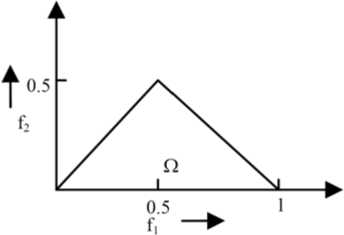
Figure 2. The usable region for calculating bispectrum

Some of these regions can be seen in (2):

Bis ( f l , f2) = Bis ( f 2 , f) = Bis ( - f l - f 2 , f2)

= Bis ( - f l - f 2 , f) = Bis ( f l , - f . - f , )          (2)

= Bis ( f 2 , - f , - f , )

The normalized bispectrum (or bicoherence) is defined as:

Bic ( f l , f2) =

Bis ( f 1 , f 2 )

V P ( f l ). P ( f2). P ( f l + f2)

Where P ( f ) is the power spectrum.

Since bispectrum and bicoherence cannot fully help signal extraction, Hinich has developed algorithms to test for non-skewness (called Gaussianity) and linearity [17]. The basic idea is that if the third-order cumulants of a process are zero, then its bispectrum is zero, and hence its bicoherence is also zero. If the bispectrum is not zero, then the process is non-Gaussian; if the process is linear and non-Gaussian, then the bicoherence is a non-zero constant [6,9].

The Gaussianity test (actually zero-skewness test) involves deciding whether the expected value of the bicoherence is zero, that is, E { Bic ( f ₁ , f ₂ )}=0. The test of Gaussianity is based on the mean bicoherence power,

S = 21 Bic (fl, f2)2 (4)

The squared bicoherence is chi-squared distributed toolbox [16]. The bicoherence was computed using the direct FFT method in the toolbox.

For the whole bifrequency plane region, four quantities were calculated: sum of the bispectrum magnitudes, sum of the squares of the bispectrum magnitudes, sum of the bicoherence magnitudes, and sum of the squares of the bicoherence magnitudes.

Since bispectrum and bicoherence are functions of f 1 and f 2 , in order to define the features, we will have five frequency intervals on each axis, as can be seen in Fig. 3. We will have 15 distinct regions. Then the defined features will be analyzed in each of these 15 regions and in the whole frequency range.

These and the three other features obtained from Hinich’s tests for Gaussian and linearity add up to make 7 features for each channel.

Рг-5	Рг-е	P2-a	Рг — Pi	Рг — Рг
Pi-8	Pi-e	Pi-a	Pi "Pi	Рг — Pi
a-S	a-0	a- a	Pi-a	Рг-а
9-6	9-6	a-9	pi-6	Рг~а
8-8	e-8	a - 8	Pi - 8	Рг " 8

Л№>

Figure 3. The different regions used for analysis in bifrequency plane

These seven features are extracted for each channel, so the total number of features by this method is: [5×4×(15+1)] + [5×3] = 335. This leads to the problem of dimensionality, which is solved by using Genetic Algorithm (GA) [18] and support vector machine (SVM) [19,20] as a features selection method. This is of interest to improve the computational speed of the classification algorithm.

( X 2 distributed) with two degrees of freedom and non

centrality parameter Lambda ( X) [16] . In (4) the squared bicoherence is the sum of P points in the non-redundant region, S is the estimated statistics for the Gaussianity test with chi-squared distributed and 2 P degree of freedom, and Pfa is the probability of false alarm in rejecting the Gaussian hypothesis. In general, Pfa is calculated as:

B. Normalization

In order to normalize the features in the limits of [-1, 1], we used (6).

Y norm

''    '

s s max s min

'

s min

^^^^^^^B

'

s max

Here Y_norm is the relative amplitude.

TO

[ e ^- t dt ,

x

'" 72(3(3

⁺ 3V P^}

More details can be found in [6,9,16].

In order to calculate these features, we used a 256

sample FFT with a default C parameter of 0.51. Based on these, the 2 P degree of freedom will be 96.

Blocks of 512 samples of EEG signals (neutral and negative), corresponding to 2 seconds, were used to compute the bispectrum and bicoherence. The analysis was done using the higher order spectral analysis ( HOSA )

• C.    Features selection

The problem of vast number of features is solved by using Genetic Algorithm as a feature selection method. The genetic algorithm is a type of natural evolutionary algorithm that models biological process to optimize complex cost function by allowing a population composed of many individuals to evolve under specific rules to a state that maximizes the fitness. The emphasis on using the genetic algorithm for feature selection is to reduce the computational load on the training system while still allowing near optimal results to be found relatively quickly. The classification performance of the trained network using the whole dataset was returned to the GA as the value of the fitness function, Fig. 4.

Classification Accuracy

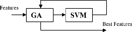
Figure 4. Combination of GA and SVM to achieve the best features

Bispectrum estimated via the indirect method

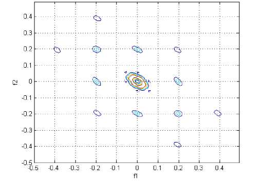
Figure 5. A contour plot of the magnitude of the indirect estimated bispectrum on the bifrequency plane, for FP1 in calm state

The GA uses populations of 100 sizes, starting with randomly generated genomes. The probability of mutation was set to 0.01 and the probability of crossover was set to 0.4. The outlet of best features using GA is consist of: sum of the sqaure of the bispectrum magnitude in alpha-alpla part, sum of the bispectrum magnitude in alpha-theta part, sum of the bispectrum magnitude in all frequency plane, sum of the bicoherence magnitude in theta-tetha part, sum of the bicoherence magnitude in beta1-alpha part.

Bispectrum estimated via the indirect method

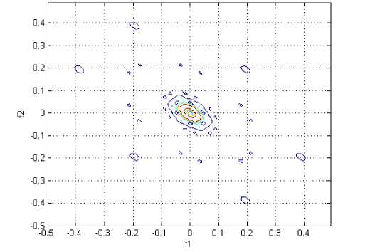
Figure 6. A contour plot of the magnitude of the indirect estimated bispectrum on the bifrequency plane, for FP1 in negative emotion

• D.    Classification with LDA

After extracting the obtained good features, we still have to find the related emotional state in the EEG. A classifier will do this process. One very useful classifier is Linear Discriminant Analysis (LDA). This procedure generates a discriminant function based on linear combinations of the features that provide the best discrimination between two different groups. It is the first proposed item for classification problems because of its simple performance and independence of several parameters adjustments. This method has been implemented on the features matrix with using SPSS software.

• IV.    Results

We used a 2-second rectangular window without overlap for data segmentation. We used around 65% of the data for training, 25% of the data for testing. The last 10% was used for validating the data. The system was tested using the 4-fold cross-validation method, which divides the training data into four parts. This method reduces the possibility of deviations in the results because of the distribution of training and test data, and ensures that the system is tested with different samples from those it has seen for training. Using a 4-fold cross validation error assessment for training and testing, we reached an average accuracy of 17.3% for the two categories of emotional states using the EEG signals. The contour plots of the Indirect Estimate of the bispectrum are shown in Figs. 5-14. According to this Figs the phase-coupled bispectrum, however, is capable of detecting and quantifying phase coupling. Therefore, the bispectrum is very useful for analyzing non-Gaussian signal such as EEG, and detecting the quadratic phase coupling between distinct frequency components in EEG signal.

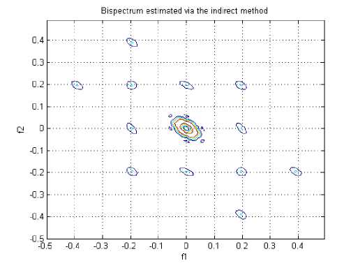
Figure 7. A contour plot of the magnitude of the indirect estimated bispectrum on the bifrequency plane, for FP2 in calm state

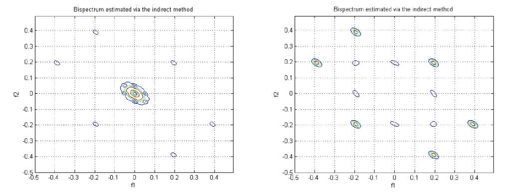
Figure 8. A contour plot of the magnitude of the indirect estimated bispectrum on the bifrequency plane, for FP2 in negative emotion

Figure 11. A contour plot of the magnitude of the indirect estimated bispectrum on the bifrequency plane, for T4 in calm state

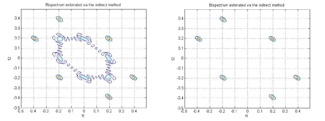
Figure 9. A contour plot of the magnitude of the indirect estimated bispectrum on the bifrequency plane, for T3 in calm state

Figure 12. A contour plot of the magnitude of the indirect estimated bispectrum on the bifrequency plane, for T4 in negative emotion

Bispectrum estimated via the indirect method

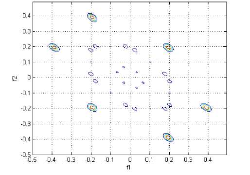
Figure 10. A contour plot of the magnitude of the indirect estimated bispectrum on the bifrequency plane, for T3 in negative emotion

Bispectrum estimated via the indirect method

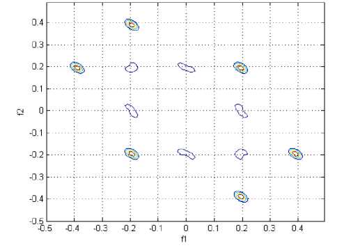
Figure 13. A contour plot of the magnitude of the indirect estimated bispectrum on the bifrequency plane, for Pz in calm state

Bispectrum estimated via the indirect method

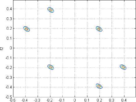
Figure 14. A contour plot of the magnitude of the indirect estimated bispectrum on the bifrequency plane, for Pz in negative emotion

The classification results of the EEG signals using LDA under two emotional states and 4–fold cross validation are given in Table 1.

TABLE I.     Emotion classificaion accuracy on eegsignals using LDA

Classifier accuracy	82.32%
4-fold cross validation-error	22.6%

Table 2 gives the average classification accuracy in five channels of EEG signals under two emotional states using LDA classifier.

TABLE II. THE AVERAGE CLASSIFICATION ACCURACY IN different channels using LDA

Channels	FP1	FP2	T3	T4	Pz
Classifier accuracy	81.2%	78%	82.3%	79.7%	75.5%

• V.    Discussion and Conclusion

This paper proposes an approach to classify emotional states in the two main areas of the valance-arousal space by using EEG signals. As demonstrated in this paper, EEG signals can be used for emotion assessment. For the first time in this investigational field, we had done a feature extraction using higher order spectra in emotional state assessment. The bispectrum is very useful for analyzing non-Gaussian signal such as EEG, and detecting the quadratic phase coupling between distinct frequency components in EEG signal. The review of the contour plots of the five channels (FP1, FP2, T3, T4 and Pz) shows that most of the changes are amplification or diminish of the peaks or transfer of the peaks in the bifrequency plane.

The best accuracy was obtained when we used the LDA, in which case the averaged accuracy was 82.32%. The classification of results demonstrated that this recognition method has a good accuracy. We concluded that HOS analysis could be an accurate tool in the assessment of human emotional states. A natural result is that it can be a good tool in the assessment of the behavior of human brain in emotional states.