Classification of Epileptic EEG Signals using Time-Delay Neural Networks and Probabilistic Neural Networks

Published Online May 2013 in MECS                                       and Computer Science

The idea of the association of epileptic attacks with abnormal electrical discharges was expressed by Kaufman [1]. Often the onset of a clinical seizure is characterized by a sudden change of frequency in the

EEG measurement. It is normally within the alpha wave frequency band with a slow decrease in frequency (but increase in amplitude) during the seizure period. It may or may not be spiky in shape. Sudden desynchronization of electrical activity is found in electrodecremental seizures. The transition from the preictal to the ictal state, for a focal epileptic seizure, consists of a gradual change from chaotic to ordered waveforms [2]. It has shown that the amplitude of the spikes does not necessarily represent the severity of the seizure.

It is now known, however, that seizures are the result of sudden, usually brief, excessive electrical discharges in a group of brain cells (neurons) and those different parts of the brain can be the site of such discharges [2].

A large number of studies aimed at classification, detection, and prediction of epileptic signals. The idea of applying neural networks for medical pattern classification has met the favour of many researchers ^{[3] [4]}. It has been noticed that the accuracy of classification entirely depends on the selected features to be applied on the EEG time series ^[5-12] .

Researchers have tried to highlight different signal characteristics within various domains and classify the signal segments based on the measured features. For example, in one study [13], the implementation of recurrent neural network (RNN) employing eigenvector methods is presented for classification of electroencephalogram (EEG) signals.

Neural Networks

Since the dynamics of the brain system are chaotic, nonlinear methods have been applied to the analysis of EEG signals [14] [15]. Nigam and Graupe [7], described a method for automated detection of epileptic seizures from EEG signals using a multistage nonlinear pre-processing filter in combination with a diagnostic ANN. Kannathal et al. [5], have shown the importance of various entropies for detection of epilepsy. Ocak [16] introduced detection of the epileptic seizures using discrete wavelet transform and approximation entropy. Ubeyli and Guleri [12], evaluate the classification capabilities of the Elman RNNs, combined with Lyapunov exponents, on the epileptic EEG signals.

In the present article, the performance of time delay neural network (TDNN) and probabilistic neural networks (PNN) on electroencephalogram signals in normal subjects and epileptic patients are investigated by using Lyapunov exponents and entropy.

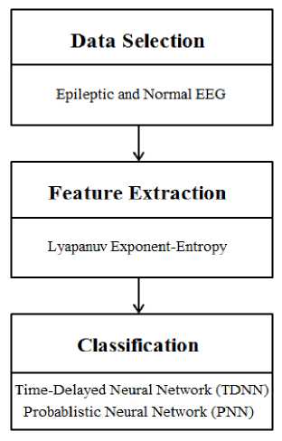
The outline of this study is as follows. In the next section, the set of EEG signals used in this study is briefly described. Then, the proposed algorithm is presented in order to classify epileptic and normal EEG waveforms. In this algorithm, Lyapunov exponents and Entropy are extracted from EEG signals and are input into the TDNN and PNN. Finally, the results of the present study are shown and the paper is concluded. Fig. 1 demonstrates the framework of the proposed method. These steps are discussed in more detail in the following sections.

• II.    METHODS

  • 2.1    Data selection

Five sets (denoted A–E) each containing 100 single channel EEG segments of 23.6-sec duration, were collected by Andrzejak et. al. [17] [18]. These segments were selected and cut out from continuous multichannel EEG recordings after visual inspection for artifacts, e.g., due to muscle activity or eye movements.

Sets A and B consisted of segments taken from surface EEG recordings that were carried out on healthy volunteers using a standardized electrode placement. Volunteers were relaxed in an awake state with eyes open (A) and eyes closed (B), respectively. Sets C, D, and E originated from EEG archive of presurgical diagnosis ^[17] [18] .

Segments in set D were recorded from within the epileptogenic zone, and those in set C from the hippocampal formation of the opposite hemisphere of the brain. While sets C and D contained only activity measured during seizure free intervals, set E only contained seizure activity. Here segments were selected from all recording sites exhibiting ictal activity.

All EEG signals were recorded with the same 128-channel amplifier system, using an average common

Neural Networks reference [omitting electrodes containing pathological activity (C, D, and E) or strong eye movement artifacts (A and B)]. After 12 bit analog-to-digital conversion, the data were written continuously onto the disk of a data acquisition computer system at a sampling rate of 173.61 Hz. Band-pass filter settings were 0.53–40 Hz (12 dB/oct) [17] [18] .

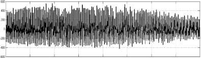
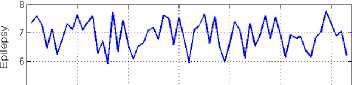
In this study, EEG signals from sets A and E were used in order to classify normal EEG and seizure activity. These two types of signals are shown in Fig. 2.

EEG signals of healthy volunteer with open eyes

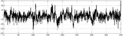
EEG signal during seizure activity

0          500         IUD         13Я         ЮЗ        2530         ИВ        Э5Ш         ЮТ

Figure2. Electroencephalographic signals. (top) Healthy volunteer with open eyes. (bottom) Epileptic patients during seizure activity.

bounded dynamical system is widely used. To discriminate between chaotic dynamics and periodic signals Lyapunov exponent (λ) is often used. It is a measure of the rate in which the trajectories separate one from other. The trajectories of chaotic signals in phase space follow typical patterns. Closely spaced trajectories converge and diverge exponentially, relative to each other. For dynamical systems, sensitivity to initial conditions is quantified by the Lyapunov exponent (λ). They characterize the average rate of divergence of these neighboring trajectories. A negative exponent implies that the orbits approach a common fixed point. A zero exponent means the orbits maintain their relative positions; they are on a stable attractor. Finally, a positive exponent implies the orbits are on a chaotic attractor ^[19] [20] .

The reason why chaotic systems, such as brain, show aperiodic dynamics is that phase space trajectories that have nearly identical initial states will separate from each other at an exponentially increasing rate captured by the so-called Lyapunov exponent.

• 2.2    Feature extraction

  2.2.2 Entropy

  
  

  2.2.1 Lyapunov exponents

  
  

  Consider two (usually the nearest) neighboring points in phase space at time 0 and at a time t, distances of the points in the i th direction being ||8x i ( 0 )| and ||8x i ( t )| , respectively. The Lyapunov exponent is then defined by the average growth rate λ_i of the initial distance

  
  

  II 8 x i ( tl

  II 8 x i ( 0 )|

  
  

  = 2^ t

  
  

  ( t ^ да )

  
  
  
  

  X i = lim -log 2 w^ t

  
  

  II 8 x , ( t 1

  II 8xi ( 0 )|

  
  

  An exponential divergence of initially nearby trajectories in phase space coupled with folding of trajectories, ensures that the solutions will remain finite, and is the general mechanism for generating deterministic randomness and unpredictability. Therefore, the existence of a positive λ for almost all initial conditions in a

  
  

  There are a number of concepts and analytical techniques directed to quantifying the irregularity of stochastic signals. One such concept is Entropy. Entropy, when is considered as a physical concept, is proportional to the logarithm of the number of microstates available to a thermodynamic system, and is thus related to the amount of disorder in the system. For information theory, Entropy is first defined by Shannon and Weaver in 1949 ^[21]. In this context, Entropy describes the irregularity, unpredictability, or complexity characteristics of a signal.

  Shannon ^[22] developed a measure to quantity the degree of uncertainty of a probability distribution. Denoting ShEn as Shannon's Entropy measure, its formal expression in the case of discrete probability distributions

  
  

  is

  ShEn = ^ P i log p i i

  
  
  
  

• 2.3    Classification

• 2.3.1    Time delay neural networks (TDNN)

Neural Networks where pT = [p1, ... , pN] is a probability distribution (superscript T represents vector/matrix transposition).

In order to compare the performance of the different classifiers, the TDNN and PNN are implemented for the same classification problem.

PNN is simpler than TDNN to implement [23]. All its connections are in the forward direction [24]. No derivatives are calculated. The training stage is accomplished in only one forward pass. Therefore it is faster in training. In addition, in probabilistic neural network the weights between the input and pattern layers are calculated directly from the training samples. Therefore, the training time of the network is generally a few seconds.

The TDNN training consists of an iterative process where each cycle consist of one or more forward propagations through the network, and one backpropagation to obtain derivatives of the cost function with respect to the network weights. In this network, the training is an iterative process. The number of iterations varies from tens to several thousands. Every iteration includes one backpropagation and one or more forward propagations for the line minimization required by the conjugate gradient algorithm [23]. When training in the batch mode, it is required to repeat the above iterations for all the training patterns in every cycle. In this network, the training speed depends on the number of training patterns and on the network's size.

TDNN typically has three layers: an input layer, a hidden layer, and an output layer. A TDNN embeds time delays on the inputs in a parallel fashion [25].

TDNNs rely mainly on special kind of memory known as tap delay line where the most recent inputs are buffered at different time steps. Such delay lines between hidden and output layers are necessary to supply the network with additional memory. In other words, by using delay lines the inputs arrive hidden layers at different points in time, so they stored long enough to support subsequent inputs.

A typical tap delay line is illustrated in Fig. 3. The response of this kind of networks in time t is based on the inputs in times (t-1), (t-2), …, (t-D). A mapping performed by the TDNN produces a y (t) output at time t as:

y (t) = f (x (t), x (t -1),..., x (t - d))

where x(t) is the input at time t and D is the maximum adopted time-delay. TDNN is well suited in the applications of time series classification.

Although all the connections in the TDNN are feedforward ^[24], which is similar to multilayer perceptron (MLP), the inputs to any unit in the network have the output of the previous stage. The activation of the unit f at any time step is calculated as follows:

i-I d yt = fixyt- k

( j = 1 k = 0

'

• ® ^ijk )

where y t is the output of node i at time t and ^ is the weight to the node i from the output of node j at time t-k [26]

Figure3. Tapped delay line memory model.

Focused Time Delay Neural Networks

Focused Time Delay Network is a MLP with a tapped delay line (also called memory layer) as input layer. A typical diagram of focused time delay neural network is illustrated in Fig. 4. This network belongs to a class of

Neural Networks dynamic networks. Delay time line is used to store the historical samples of the inputs. The number of historical samples determines the size of the memory layer to express the features of the input in time. The memory is always at the input of multilayer feed-forward networks; hence the name focused comes.

Training in focused time delay network is much faster than other dynamical network for two reasons: firstly, as mentioned before, tapped delay appears only at the input layer and secondly, the loop does not contain feedback connections or adjustable parameters. For that reasons, no dynamic back propagation are needed to compute the network gradient. It can still be trained with static back propagation [27] [28].

A TDNN can be used for either function estimation or function prediction in addition to classification or classification prediction [25].

• 2.3.2    Probablistic Neural Networks Classifier

A probabilistic neural network is also good for classification problems [29]. When an input is feed into the classifier, the first layer will be able to compute the distance between the input vector and the training input vectors, and produce a vector whose elements show the closeness between the input data points and the training vector points [30].

The second layer will sum up “contributions for each class of inputs to produce as its net output a vector of probabilities.” As the last step, a transfer function called “compete” will pick the maximum of the probabilities on the second layer, and it will also provide a one for that class and a zero for the other

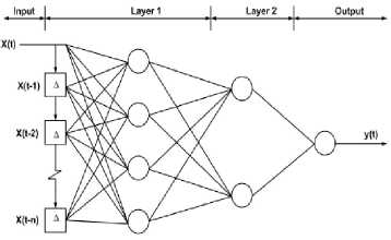
Figure4. Focused time delay neural network with two layers.

classes [30]. The probabilistic neural network architecture is shown in Fig. 5.

The training process of a PNN is essentially the act of determining the value of the smoothing parameter, sigma. An optimum sigma is derived by trial and error.

Like the other neural networks, the usage of this network has some advantages and disadvantages. Probabilistic neural networks (PNN) can be used for

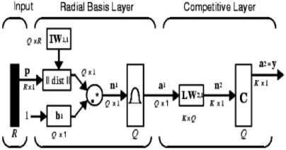
Figure5.Probabilistic Neural Network architecture ^[31] .

classification problems. Their design is straight-forward and does not depend on training. A PNN is guaranteed to converge to a Bayesian classifier providing it is given enough training data. These networks generalize well.

The PNN have many advantages, but it suffers from one major disadvantage. They are slower to operate because they use more computation than other kinds of networks to do their function approximation or classification.

• III.    EXPRIMENTAL RESULTS

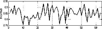
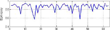
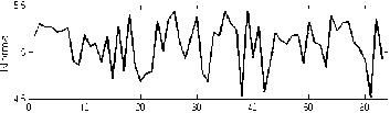
The values of the maximum Lyapunov exponents are given in Fig. 6. According to the results, all the Lyapunov exponents are positive, which confirm the chaotic nature of the EEG signals in both groups. Fig. 7 depicts the Entropy values of EEG signals in normal and epileptic subjects.

In the next stage, Lyapunov exponents and Entropy are used as inputs of the TDNN and PNN classifiers. In order to classify EEG signals with TDNN, different network architectures are tested. The number of output is 2 with target outputs of normal and partial epilepsy.

Neural Networks

Lyapunov Exponents

Subject

According to Table I, the best classification result of TDNN is achieved by 12 neurons in the hidden layer, with the training time of about 19.69 seconds. Classification result for the test data is shown in Fig. 8.

Classification result for test data

• 3|                  ,                ,        ---------T-----------------I-----------------T-----------

• System Output :         ;

  -------Desired Output :          ^:          .

Figure6. Lyapunov exponent of EEG signals: (top) normal, (bottom) partial epilepsy.

Entropy

5o 10          20          30          40          50 GO

Subject

Figure7. Entropy of EEG signals: (top) normal, (bottom) partial epilepsy.

In this application, in the hidden layer, hyperbolic tangent sigmoid transfer function is used as activation function and in the output layer, linear transfer function is applied. Delay vectors are adjusted to be 0-5 and 0-3 in the first and second layers, respectively.

The extracted features are randomly divided into two sets: a training set and a testing set. 2/3 of the samples are used to train the classifiers while 1/3 is used to test the performance of each classifier. The values of the central processing unit (CPU) times of training and the classification error (mean square error) of TDNN are presented in Table I.

TABLE I. The values of mean square error and the CPU times of training of the TDNN classifier.

Classifier	Neurons in hidden layer	MSE	Elapsed time (s)
TDNN	3	8.43×10 -15	14.57
	5	6.86×10 -15	14.78
	8	5.22×10 -15	16.09
	12	2.25×10 -15	19.69
	14	1.01×10 -14	36.03

• 1--:------------;------------—1........i............:  -

• 0.5 -...........i............i...........;............i............I............j-

  • °0       10      20      30      40      50      6070

Figure8. TDNN out put with 12 neurons in the hidden layer (black and green curves show the desired outpout and sysyem output, respectively).

As mentioned before, in order to study the performance of probabilistic neural network, the same features are used as an input.

In the study of probabilistic neural network, an optimum sigma is derived by trial and error. Systemic testing of values for sigma over some range can result in bounding the optimal value to some interval.

The effect of sigma on classification rate is evaluated. Fig. 9 shows the effects of different sigma on the classification accuracy rate.

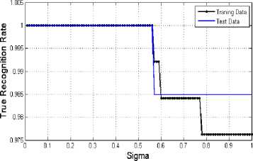
Figure9. The effect of different sigma on correct classification rates.

As shown in Fig. 9, the best result of classification is achieved by sigma < 0.56. Classification result (with sigma=0.56) for test data is shown in Fig. 10. As this figure shows, by choosing sigma=0.56, 65 samples from 66 test samples are recognized as true class and only one sample is recognized as false class.

Neural Networks

System Output -----Desired Output

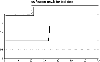
Figure10. PNN output with parameter sigma=0.56 (black and green curves show the desired outpout and sysyem output, respectively).

• IV. CONCLUSIONS

In order to reduce the time and physicians’ mistakes, automatic computer based algorithm have been proposed to support the diagnosis and analysis performed by physician [32].

Various methodologies of automated diagnosis have been adopted; however, the entire process can generally be subdivided into a number of disjoint processing modules: data collection/ selection, feature extraction/ selection, and classification.

The main goal of this study is to evaluate the diagnostic performance of TDNNs and PNNs with Lyapunov exponents and Entropy on EEG signals in epileptic patients. Decision making was performed in two stages: Feature extraction and classification using classification on the extracted features.

In order to classify EEG signals (EEG recordings that were carried out on healthy volunteers and epileptic patients during seizure activity), an application of TDNN and PNN employing nonlinear features was presented.

Nigam and Graupe [7], proposed a method for automated detection of epileptic seizures from EEG signals and the total classification accuracy of their model was 97.2%. Guler et al. [33] evaluated the diagnostic accuracy of the recurrent neural networks (RNNs) employing Lyapunov exponents trained with Levenberg-Marquardt algorithm on the same EEG data set (sets A, D, and E) [17] [18] and the total classification accuracy of that model was 96.79%. In another study [34], it is found that among the different entropies applied, the wavelet entropy features with recurrent Elman networks yields 99.75% and 94.5% accuracy for detecting normal compare to epileptic seizures and interictal focal seizures, respectively. Ocak [16] reported that by using approximate entropy (ApEn) and discrete wavelet transform (DWT) analysis of EEG signals seizures could be detected with over 96% accuracy.

To evaluate the performance of the classifiers, mean square error and the CPU times of training were examined. The results of the present study demonstrate that the best classification result for TDNN is achieved with 12 neurons in hidden layer. Training time of the experimentation is about 19.69 second with 12 neurons in hidden layer.

In the study of probabilistic neural network, it has been shown that the sigma values which are lower than 0.56 have better performance in the proposed network structure. Previously, it has been shown that the training time of the network is generally a few seconds [23]. The results of this study also confirmed it as the CPU times of training for PNN with sigma=0.56 is about 0.87 s.

The results of present study showed that applying nonlinear features to train these networks can serve as useful tool in classifying the EEG signals.