Classification of Non-Proliferative Diabetic Retinopathy Based on Segmented Exudates using K-Means Clustering

Published Online December 2014 in MECS

Diabetic retinopathy is one of severe complication diseases caused by long term suffering of diabetes mellitus. For a person under 30 years old with diabetes mellitus, the probability of suffering diabetic retinopathy is approximately 50% and 90% after 10 and 30 years, and approximately 5% for type 2 diabetic persons [1]. Without treatment, this disease may cause blindness. The existence of hard exudates shows that a patient has diabetic retinopathy. Hard exudates marked by bright spots consist of yellow deposits of lipids and protein that leaks from the blood vessels. Since hard exudates start appear in the early stage. Generally, an ophthalmologist evaluates hard exudates to diagnose the severity degree of the disease, which can be subjective and time consuming.

This research automates the segmentation of hard exudates to obtain a more accurate and faster evaluation process.

Diabetic retinopathy starts with the small changes in retinal capillaries. When microaneurysms are detected as dark/red small dots in the retina, this disease is catagorised as mild Non-Proliferative Diabetic Retinopathy (NPDR), hemorrhage might happen because of the weakness of small capillarity, located near microaneurysms [2]. Then emerge retinal edema and hard exudates followed by capillar wall leakage [3]. In moderate NPDR, there are often exist microaneurysms in the middle of the hard exudate ring. The blokage of the blood vessel cause microinfarcts which is called soft exudates or cotton wool. In the stage of severe NPDR, the number of hemorrhages, soft exudates, microvascular increases and the extensive lack of oksigen can change the condition becomes proliferative diabetic retinopathy which forms neovascularisation. At the end, this abnormality may cause retinal detachment. Fig. 1 illustrates a retinal fundus image with diabetic retinopathy. The retina structure consists of blood vessels, optic disc, and macula [4].

There are previous studies to clasify the stages of NonProliferative Diabetic Retinopathy (NPDR) and Proliferative Diabetic Retinopathy (PDR) based on areas and blood vessel perimeters using Back Propagation Artificial Neural Network [5, 6]. Several studies use the features of hard exudates for the classification models. One study utilize the similarity measure with the mean and median values as features [7].

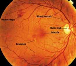
Fig. 1. A retinal fundus image with diabetic retinopathy [4].

There are different methods for exudate segmentation, those are Fuzzy C-Means Clustering with spatial correlation [8], the adaptive region growing method [9], and the morphology approach [10]. There is also a study employs four features derived from the exudate segmentation for classification [11].

In this study, the applied method is based on K-means clustering and the feature vector of the segmented exudates is classified using three different classifiers to get comparison of results.

This paper has five parts, the first part gives a brief description of diabetic retinopathy development and the previous studies of exudate detection and NPDR classification. The second part explains the methods used in this research, which consists of the mathematical morphology, K-Means clustering, SVM and its soft margin, Multilayer Perceptron, and Radial Basis Function Network. The third part illustrates the design and the implementation of the system. The two last parts give the results and analysis, and the conclusion of the study.

• II.    Background

• A.    Morphological Contrast Enhancement

This method is a combination of two methods, namely morphological Top-Hat and Bottom-Hat Transform. The process of image enhancement is given by the following equation:

fl = + У th ⁽А)- Фтн ( fi ) (1)

Image f2 is the result of image enhancement and image f1 is the input image of the process.

The results of the Top-Hat Transform У th is the bright areas of the image f₁ and the results of the Bottom-Hat Transform Фтн is the dark areas of the image f₁.

• B.    Top-Hat and Bottom-Hat Transformation

Top-Hat Transform or Top-Hat by Opening is defined as the difference between the input image and the result of the opening of the input image by a structuring element. The equation of the Top-Hat Transformations are as follows:

Bhat ( f )= f -( f ^∘ b ) (2)

Bottom-Hat or Top-Hat by Closing is defined as the difference between the input image and the result of closing the input image itself. Equation of Bottom-Hat Transformations expressed as follows:

Bhat ⁽ f )=( f ^∙ b )- f (3)

• C.    K-means clustering

K-means is a common algorithm for clustering. In image segmentation it finds its application in clustering pixels according to the grayscale values. The membership for each pixel belongs to its nearest center, depending on the minimum distance.

The steps for K-means clustering algorithm consists of initializing K center points, computing the distances between each point and the center points, and determining the membership based on the minimum distance. Afterward the center points are updated. This process is iterated until all memberships are settled. There are several modification of K-means clustering concerning the center points initialization selection.

In this research, the initialization of the K center is performed randomly. K points of the data are chosen randomly as K centers. Once the K center points for K clusters are chosen, the next step is grouping each other points into a specific cluster. The point will be grouped into a cluster if the point is closest to the the centroid of the cluster. In order to determine the closest centroid, the Euclidean distance is employed. The Euclidean distance is defined in the next formula:

Euclidean distance = √∑ (^ - Ci )⁵ (4)

In (4), p is a point and c is a centroid. Either a point or centroid has dimension n.

When all of the points have been assigned into clusters, the next step is updating the centroid of each cluster. The updated centroid is computed as the mean of the member points in a cluster (5). In (5), c_i is the centroid of the i-th cluster, m_i is the number of member points in that cluster, and p is the member point in the cluster.

Ci _{= ∑} p ∈ cP (5)

After all centroids are updated, the process of points assignment to the clusters is repeated using Euclidean distance (4). The iterative process is terminated when the centroid for each cluster is unchanged. Another termination process is based on the maximum number of iteration. The algorithm of the K-Means Clustering is summarized in Fig. 2.

• D.    Support Vector Machine

The purpose of Support Vector Machine is finding the best hyperplane that serves as a separator of the two classes in the input space, namely class -1 and class +1. The best hyperplane separates two classes at maximum margin (Fig. 3).

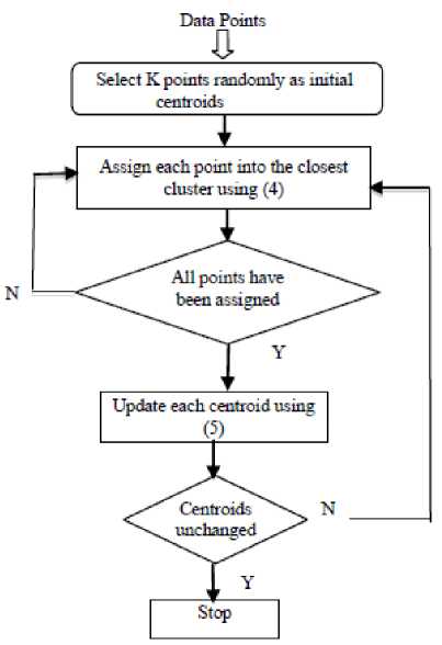
Fig. 2. K-Means Algorithm.

The margin is the distance between the hyperplane with the nearest data from each class. The closest data is referred to as support vector [12]. The training dataset is defined as ∈ with label ∈ {-1,+1}, =1,…, . The hyperplane function is represented as follows,

( )=  .  +  =0(6)

Where, = , ,…, is a weighting vector and b is a bias [12]. To maximize the margin, we should solve the following minimization problem as follows:

‖   ‖(7)

subject to ( +   )≥1, =1,…,.

The problem is solvable if the data is linearly separable.

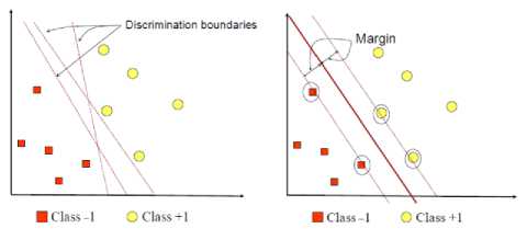
Fig. 3. Finding optimum hyperplane with SVM [12].

However, if soft margin SVM is employed, some misclassified data are allowed by modifying the minimization problem with an additional term represented by a slack variable such that the problem becomes:

( )=  ‖  ‖ +  ∑ ℰ     (8)

subject to ℰ ≥0

( +   ) ≥1-ℰ, =1,…, .     (9)

The slack variable value for data between the margin is 0≤ℰ ≤1 . The data with the slack variable value ℰ ≥1 are incorrectly classified. The score of C defines the trade-off between maximum margin and the error that can be tolerated.

The optimization problem is solved by applying the Lagrange multiplier ∝≥0, =1,…,  . The solution equation for the optimization problem is given by [12]:

n w=Li=1ai. y. xi

En a. y t = о.

The value of b is calculated as follows:

( +   )=(1-ℰ)

=  (1-ℰ )-(  )(11)

• E.    Multilayer Perceptron

One of Artificial Neural Network variants is Multilayer Perceptron (MLP) [13]. The architecture of MLP consists of at least three layers: input, hidden and output layer. In the training stage, the model compute weights of the networks. The computed weights will be used to classify the class of query data in the testing stage. In the training stage, the model computes weights using feed forward propagation and back propagation algorithm. The architecture of the three layers MLP is depicted in Fig. 4.

In Fig. 4, the input layer consists of n nodes (x₁...x_n-1). The hidden layer (Oh₁...Oh_m) consists of m nodes and the output layer consists of one node (O_k). The weights from an input node to a hidden node is denote as w_ih. In order to differentiate between one weight with another, an index is used. For example, w ih[11] means the weight connect the first node at input layer and the first node at the hidden layer. In addition, the weights from hidden units to output units are denote as w hk . The same indexing is applied as in the w ih . At the beginning of the training stage, all weights are initialized randomly. The value of the nodes in the hidden layer (Oh₁...Oh_m) and the value of O_k are computed using the feed forward propagation algorithm. The formula for computing each O_h and O_k are defined in (12) and (13).

ℎ=           (∑      ․  )           (12)

=             (∑       ․ ℎ )          (13)

There are several activation functions (denote as ActivFunct() in the (12) and (13)). The activation function used in this research is Sigmoid function (14).

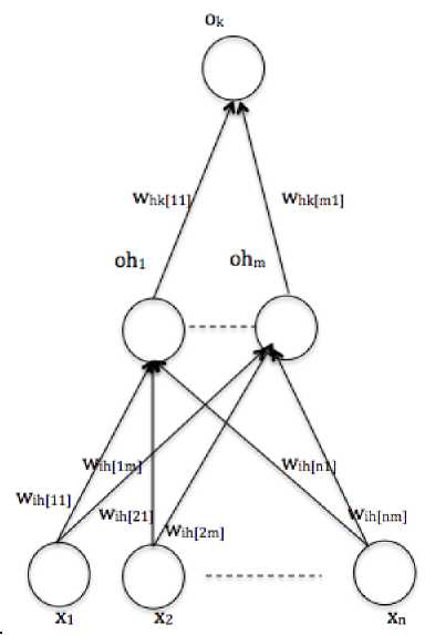
Fig. 4. Architecture of Multilayer Perceptron.

The y value in (14) is the dot product of w_ih vector and x vector. Similarly, for the output unit, y is the dot product of w hk vector and [Oh 1 ,...,Oh m ].

5 igm о id = ^__y (14)

In order to update all weights in the network, the model perform the back propagation algorithm. The algorithm is based on error correction in O h and O k . Error in the hidden layer and error in the output layer are computed according to (15) and (16) respectively.

δ = o (1 - o )( t  - o )

k  k   kk  k

δh =oh(1-oh)   ∑ k ∈output

w  ⋅δk hk

In the (15), k_k, k_k,k_k are the error of the ouput layer, the output layer value and the target value respectively. The target value is the real class of each point data. In (16), 5_k, o_k, w_kk are the error of the hidden layer, the output of hidden layer and the weight between the hidden layer and the output layer.

The next step in the training stage is updating the w ih and updating w hk . The updating process involve error in the hidden layer (15) and error in the output layer (16). The update computation of weights (w_ih and w_hk) are based on the following equations.

w_ih = w_ih + T]6_hx_t                (17)

w_hk = w_hk + g 5 oO _h i               (18)

In (17) and (18), g denotes the learning rate. The updating weights in the training stage that involve feed forward propagation and backpropagation are iterated until meet the stopping criterion. The stopping criterion could be based on convergence (the errors unchanged) or based on epoch (maximum iteration).

At the prediction stage, a query data will be classified as moderate NPDR or severe NPDR. In order to predict the query data, the trained model will perform feed forward propagation. The feed forward propagation involves the result of wih and whk that are obtained from the training stage. Once the output of the network (Ok) is calculated using (13), the output value is processed using Sigmoid Activation function (14). The class determination using threshold for the ouput value. If the value less than 0.5, the class of query data is classified as moderate NPDR. Otherwise, the class of query data is classified as severe NPDR.

• F.    Radial Basis Function Network (RBFNN)

Another variant of the Neural Network is Radial Basis Function Network (RBFNN) [13]. The RBFNN can involve the supervised and unsupervised training. The architecture of the RBFNN is similar to the architecture of the MLP. However, the hidden layer do not involves the Activation Function. The hidden layer states the Radial Basis Function (RBF). The weights from the input layer into the hidden layer are represented as the centres of the RBF (g _i )\

In order to determine the centres of the RBF, the model could perform the unsupervised learning. For example, K-Means clustering is performed before training a network model. Subsequently, the centroids of clusters from K-Means algorithm will be used as the centres of the RBF. The centres of RBF replace the w_ih in MLP. Once the centres are determined, the weights from nodes in the hidden layer and the nodes in output layer (w hk ) are initialized randomly.

Then the training process is continued with supervised learning. The supervised learning process similar to the learning process in MLP. There are two choices when design the next learning process. Firstly, the centers of the RBFs are fixed and the learning process only update the w_hk. Secondly, the learning process update both center of RBFs and the (g_ik) and w_hk. In this research, the first learning process is chosen. The architecture of the RBFNN is ilustrated in Fig. 5.

Similar to MLP, the supervised learning includes feed forward propagation and back propagation. In the feed forward propagation, the output of nodes in hidden layer (Oh 1 ...Oh m ) and the output of nodes in output layer (O k ) are computed. Different to MLP, the computation of output of hidden layer nodes are based on the following equation:

0 h = e"(^~ ф: z 2 °2) (19)

In (19), the euclidean distance between centre of the RBF function (g _i )) and the input vector is computed first. Subsequently, the computed distance is processed in the

Gaussian function. The Gaussian function has a width parameter ( a ). The nodes value of output layer nodes (O_k) is calculated from the output of the hidden nodes (O h1 ...O hm ) that are multiplied with w hk using (13). Next, the error of the output layer (5 ) is computed using (15). The error is used to update w hk using (18) in the back propagation.

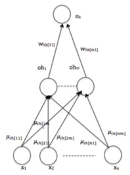
Fig. 5. The architecture of RBFNN.

The learning process (feed forward propagation and back propagation) is repeated until stopping criterion met. Similar to MLP, the stopping criterion could be determined based on epoch or the convergence of error. The result of this learning process is the model with the trained weights and the centres of the RBF function.

When predict a query data, the model will perform a feed forward propagation. The RBF centres and the updated w hk from the training stage are involved in the computation of the network output (O k ). The output of the network (O k ) is calculated using (11). Subsequently, the output value is processed using Sigmoid Activation function (14). The determination of the query data class using threshold. If the value of network output is less than 0.5, the query data is classified as moderate NPDR. Otherwise, the class of query data is classified as severe NPDR.

• III.    Design And Implementation

The detection of hard exudates consists of two stages. The flowchart of the exudates detection is shown in Fig. 6. The first stage is the preprocessing stage to prepare the image for segmentation. The input images are the retinal fundus images taken from Messidor database [14]. The original image is resized into 576 x 720 and converted into a green channel, then it is contrasted using morphological enhancement, such that the difference between the bright dan darker areas is intensified.

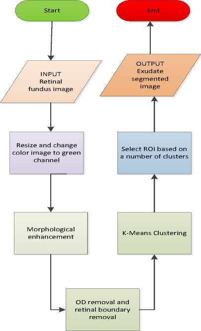
Fig. 6. Flowchart of the exudate segmentation.

Then the optic disc is eliminated by a circle centered in the cup with the diameter of the same length of the optic disc bounding box given by high grayscale values. Other methods for finding the optic disc area include the circular Hough Transform [15] and the adaptive morphological approach [16]. There are also several techniques for detecting the bright part of the retina, which covers the cup and the optic disc [17]. Besides the optic disc, the retinal boundary in some images has high grayscale that it should be detected and subtracted from the enhanced image. The second stage is the segmentation process by using K-Means Clustering to partition the retinal image into areas of the same grayscale represented by the grayscale of the clustering centers. The exudate areas are obtained by selecting 20 clusters from 32 clusters for K=32, beginning from the maximum grayscale value.

From the segmented exudates, we construct a feature vector which consists of the exudate area, perimeter, number of centroids, and the standard deviation of the centroid coordinates. The feature vector is applied to a classifier to predict the moderate or severe grading of NPDR [11]. In this study we compare three types of classifiers, those are linear soft SVM, multilayer perceptron, and RBF network.

• IV.    Results

This study uses 56 images for training data and 56 images for testing data, each consists of 20 images with moderate NPDR and 36 images with severe NPDR.

Fig. 7 – Fig.12 show the images before and after enhancing and removing OD. Fig. 13 and Fig.14 shows retinal boundary detection that subtracted from the enhanced image to remove the boundary effect on segmentation. Fig. 15 - Fig. 17 show the segmented images after K-Means Clustering with different numbers of clusters.

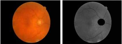
Fig. 7. Image 1 before and after enhancing and removing OD.

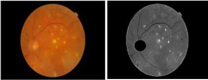
Fig. 8. Image 2 before and after enhancing and removing OD.

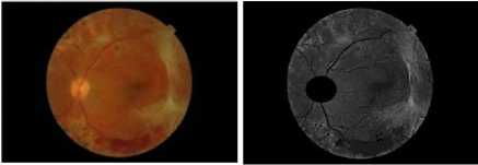
Fig. 9. Image 3 before and after enhancing and removing OD.

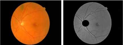
Fig. 10. Image 4 before and after enhancing and removing OD.

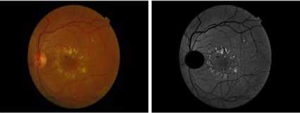
Fig. 11. Image 5 before and after enhancing and removing OD.

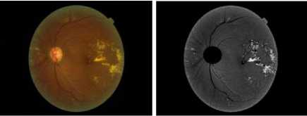
Fig. 12. Image 6 before and after enhancing and removing OD.

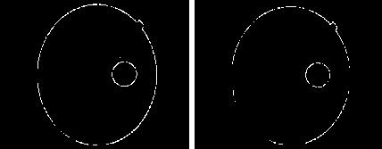
Fig. 13. Retinal boundary detection for image 1.

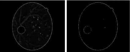
Fig. 14. Retinal boundary detection for image 2.

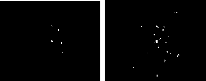
Fig. 15. Exudates of image 2 with difference number of clusters.

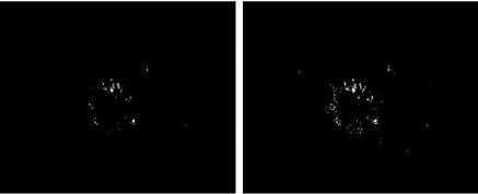
Fig. 16. Exudates of image 5 with difference number of clusters

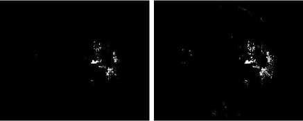
Fig.17. Exudates of image 6 with difference number of clusters.

The classification results are tabulated in Table 1. With 56 images as the testing data, soft SVM classifier , multilayer perceptron, and RBF network can classify correctly 50, 51, and 48 images respectedly, which gives the accuracy of 89.29%, 91.07%, and 85.71%.

Table 1. Classification results

No.	Classifier	Accuracy
1	SVM	89,29%
2	Multilayer Perceptron	91,07%
3	RBF Network	85,71%

• V.    Conclusion

This study proposes exudate detection, feature extraction, and the classification of NPDR severity grading. The exudate detection utilizing K-Means Clustering provides good result as an input to the classification system of NPDR. This is also supported by morphological enhancement which is able to intensify the difference between the bright dan darker areas without affecting the area sizes of different components. The exudate segmentation converts the segmented exudates into a binary image. From the binary image, a feature vector is constructed to give four attributes, those are the area sizes, perimeters, number of centroids and standard deviation of each exudate image. Finally, the feature vectors are trained and tested using three different classifiers, i.e. soft margin SVM, multilayer perceptron, dan RBF network.

The experiment results show that the three classifiers give high accuracy when classify retinal images of NPDR as moderate or severe categories, especially for multilayer perceptron. We expect this classification model can be developed further as an automation system to produce a system for supporting early detection of diabetic retinopathy efficiently.

For the future work, this research will be extended further by involving other components of diabetic retinopathy indications, such as microaneurysms and hemorrhages. There are some previous studies related to detecting the red lesions and the dark area of macula [18, 19, 20, 21]. With further study, we expect that the system can classify the grades of diabetic retinopathy in more detail evaluation.

Acknowledgment

This work is supported by the grant from Directorate General of Higher Education, Ministry of National Education and Culture, Indonesia.

Messidor database is kindly provided by the Messidor program partners (see .