Classifying Similarity and Defect Fabric Textures based on GLCM and Binary Pattern Schemes

Published Online November 2013 in MECS DOI: 10.5815/ijieeb.2013.05.04

Texture is also a main visual feature that refers to natural and fundamental surface properties of an object and their relationship with the surrounding atmosphere. It can be seen practically anywhere. The texture can be regarded as the visual look of a surface or material. Typically, textures and the analysis techniques associated with them are divided into two major categories with dissimilar computational approaches: the stochastic and the structural methods. With a very regular appearance structural textures are frequently man-maid. In structural texture analysis, the properties and the appearance of the textures are described with dissimilar policy that specify what kind of primitive elements there are in the surface and how they are located [14]. Texture classification is a primary issue in computer vision and image processing, playing a very significant role in a wide range of applications that include medical image analysis, remote sensing, object recognition, document analysis, environment modeling, content-based image retrieval and many more. The local binary pattern (LBP) is one of the most used texture descriptors in image analysis [7].

Texture provides essential information for many image classification tasks. Much research has been done on texture classification during the last three decades; most traditional approaches included gray level co-occurrence matrices (GLCM), second-order statistic method, Gauss– Markov random field, and local linear transform, which are restricted to the analysis of spatial relations between neighboring pixels in a small image region. Recently, effective measurement of local brightness variations and local texture softness by using features such as BDIP (block difference of inverse probabilities) and BVLC (block variation of local correlation coefficients) have been proposed. As a consequence, their performance is the best for the class of so called micro-textures [6] [12] .Texture classification plays an important role in the engineering fields and scientific researches. It can be used in image database retrieval, industrial, agricultural and biomedical applications as well. The training phase and testing phase/recognition phase are the two different process involved in texture image classification. In the training phase a set of known texture images are trained by feature extraction method and stored in the library or database. In the recognition phase the unknown sample image is tested by using same feature extraction method and compares the values are compared with the already stored features in the database [11].

Texture is characterized not only by the gray value at a given pixel, but also by the gray value pattern in a neighborhood near the pixel. Generally, the term texture refers to repetition of texture primitives or fundamental texture elements called texels. A texel contains a number of image pixels, whose placement may be periodic, quasi-periodic, or random. The category of the texture determined by the repetitiveness of the texels and the texture analysis approach is decided [8]. A texture image is principally a task of the subsequent variables: the texture surface, its albedo, the camera, the illumination, and its viewing arrangement. It is a mixture of all these factors which makes the texture classification a difficult task . Due to the increasing demand of such applications, texture classification has received substantial attention over the last several decades and several novel methods have been proposed [15]. One of the most important problems is that the textures in the real world are often dissimilar due to variations in orientation, size, or other visual appearance. Due to irregular illumination or large within-class inconsistency the gray-scale invariance is frequently significant. Moreover, most proposed texture measures have a high degree of computational complexity.

In various applications, to deal with the semantic gap trouble, texture features are employed. For example, it is used to explain topographical surfaces in satellite images and organ’s tissues in the medical imaging field. Thus, the majority of the research in the area of texture analysis is devoted to developing the inequitable capability of the features extracted from the image Texture analysis is typically a very lengthy practice [5]. A neural network as a classifier is used in many texture identification systems. Neural networks have been paying attention researchers in pattern recognition because of its power to learn from training dataset. An example would be the back-propagation for adaptive route selection policy in mobile ad hoc networks. PNN is another neural network that has been used in several applications. The applications are remote sensing image segmentation and surface defect identification. PNN has verified to be efficient more than conventional back-propagation and has been accepted as an substitute in realtime categorization problems [10].

In order to devise an efficient algorithm for texture classification it is necessary to find a set of texture features with good discerning power. Most of the textural features are usually obtained from the application of a local operator, statistical analysis or dimension in a transformed domain. In general, the features are predicted from co-occurrence matrices, Law’s texture energy measures, Fourier transform domain, Markov random field models, local linear transforms etc [16]. Local Binary Patterns (LBP), a non-parametric technique summarizing the local structures of an image efficiently has received growing interest for facial representation recently. LBP was initially proposed for texture description, and has been broadly exploited in numerous applications. The most important properties of LBP features are tolerance against the monotonic illumination changes and computational simplicity as well [20]. In recent years, LBP features have been extensively exploited for facial image analysis, together with face detection, face recognition; facial expression analysis, gender/age categorization and some other applications. In the meantime, different variations of the original LBP have been proposed for an improved performance.

This work addresses the above mentioned issues. In this paper, a collective methodology is proposed for both scale and rotation invariant classification. The outline of this paper is as follows. The proposed texture classification algorithm and a detailed review about the various features and classifiers considered in this work are described in Section 4. Section 5 provides a detailed mathematical model of the proposed texture classification. Section 6 illustrates the experimental results and evaluates the performance of the proposed system. Then the conclusion from this work is summarized in Section 7.Finally, the paper ends with the references.

• II.    RELATED WORK

Alireza Tavakoli Targhi et al. [19] have proposed a technique for texture classification with minimal training images. They have classified texture from a single image under unknown lighting conditions. The current and successful approach to this task is to treat it as a statistical learning problem and learn a classifier from a set of training images, but this required a not only a sufficient number but also a variety of training images. They showed that the number of training images required can be drastically reduced (to as few as three) by synthesizing additional training data using photometric stereo. They demonstrated the method on the PhoTex and ALOT texture databases. Despite the limitations of photometric stereo, the resulting classification performance surpassed the state of the art results.

Dattatraya S. Bormane et al. [1] have developed a scale invariant texture classification method based on Fuzzy logic. It was applied for the classification of texture images. Two types of texture features were extracted ; one using Discrete Wavelet Transform (DWT) and other using Co-occurrence matrix. Co-occurrence features were obtained using DWT coefficients. Two features were obtained from each sub-band of DWT coefficients upto fifth level of decomposition and eight features were extracted from co-occurrence matrix of the whole image and each sub-band of first level DWT decomposition. The fuzzy classification was achieved in two steps, fuzzification and rule generation. The performance was measured in terms of Success Rate. This study showed that the proposed method offered excellent scale invariant texture classification Success Rate. Also, wavelet features like standard deviation and combination of energy along with some proposed hybrid feature sets outperformed the other feature sets. This success rate was comparatively high when compared with results published earlier.

Jing Yi Tou et al. [17] have analyzed recent trends in texture classification in which they have aimed to compile the recent trends on the usage of feature extraction and classification methods used in the research of texture classification as well as the texture datasets used for the experiments. The study showed that the signal processing methods, such as Gabor filters and wavelets were gaining popularity, but old methods such as GLCM were still used but were being improved with new calculations or combined with other methods. For the classifiers, nearest neighbor algorithms were still fairly popular despite being simple and SVM has become a major classifier used in texture classification.

• III.    MAIN CONTRIBUTIONS

First, this work enhances the recent technique on texture classification for better dealing with rotation invariant fabric images. Binary pattern features are extracted and steering filter is applied to them at different orientations. GLCM features are then extracted and as the ultimate step, two types of classifications such as, similarity and defect classifications are performed on the input fabric texture images. Finally, our experiments with three different patterned fabric images (star, box and dot) and with the three different classifiers provide a better classification rate.

• IV.    PROPOSED METHODOLOGY

• 4.1.    Intensity Normalization

• 4.1.1.    Histogram Equalization

• 4.2.    Feature Extraction

• 4.2.1.    Binary Patterns

The proposed system for texture classification is built based on the features GLCM, LBP, LLBP, SLBP and by applying K-NN, SVM and PNN as classification algorithms. The intensity of the image is first normalized and after that, binary patterned images are constructed and a steering filter is applied at different rotational angles {0, 45,-45,180}. After the extraction of the GLCM features, similarity and defect classification is performed using classifiers like SVM,K-NN and PNN. For defect Classification, the following steps are performed. First, the defect free images of different patterns were used for training. Then the feature vectors of k x l dimensions are acquired for these images, where “k” is the number of training images and “l” is the dimension of the features. Here, different defective images like broken end, hole, thick bar, thin bar and netting multiple [2] were used for testing/classification. Similarity based classification is done by using the same steps like defect Classification.

The theoretical background of all the approaches employed and the overall processing steps are discussed in this section.

Many papers attempt to get some face feature which is insensitive to the variation in illumination. With the feature, the varying illumination on image cannot manipulate the classification result. In other words, we can eradicate the illumination factor from the image. The best way to do this is to separate the intensity information from the identity information.

The image intensity is normalized by applying a technique called histogram equalization which is described as follows.

Histogram equalization (HE) is a classic technique. It is generally used to make an image with a uniform histogram, which is considered to produce an optimal global contrast in the image. However, HE may make an image under irregular illumination to be more irregular. S.M. Pizer and E.P. Amburn (Pizer & Amburn, 1987) proposed adaptive histogram equalization (AHE). It calculates the histogram of a local image region centered at a given pixel to determine the mapped value for that pixel; this can accomplish a local contrast enhancement.

Feature Extraction is a major process in all classification and recognition applications. For texture classification several feature extraction methods are available. Few of them are Binary patterns, GLCM, GLWM, TGF, DBWP etc. Our proposed texture classification considers two feature types, such as GLCM and binary patterns which are detailed in the following sub sections.

Binary pattern is an image formed by a formula that consists of binary operations and results in a 32-bit integer number. These patterns are closely united to the 32-bit RGB color system. Any integer numbers can use these patterns . The different binary patterns considered in this work are Local Binary Pattern (LBP) , Simplified Local Binary Pattern (SLBP) and Local Line Binary Pattern (LLBP).

• 4.2.1.1    LBP

• 4.2.1.2.    SLBP

• 4.2.1.3.    LLBP

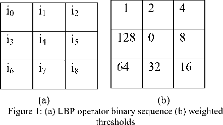
The local binary pattern (LBP) texture analysis operator is defined as a gray-scale invariant texture measure derived from a common definition of texture in a local region. It is an effortless but efficient texture operator which labels the pixels of an image by the process of thresholding the neighborhood of each pixel and results a binary number. It became an admired technique due to its discriminative power and computational simplicity [4]. Ever since the LBP was, by definition, invariant to monotonic alterations in gray scale, it was incremented by an orthogonal assessment of local contrast. Fig 1 shows how the contrast measure (C) is derived. The gray level average below the center pixel is subtracted from that of the gray levels that are above the center pixel. The LBP and local contrast measures are used as two dimensional distribution features.

Simplified local binary pattern (SLBP) was proposed by Qian Tao and Reymaond Veldhuis for illumination normalization. This is calculated by allotting equal weights to each of the 8 near regions. SLBP shows that the processed image becomes more robust to illumination changes. It has the following merits: the simplified one is not directional-sensitive and the coding number is largely reduced from 256 to 9 patterns.

Local line binary pattern (LLBP) is derived from local binary pattern (LBP) and it reveals the local spatial structure of an image by the process of thresholding. The texture presentation denoted as decimal number is initiated from the local window with binary weight. LLBP has a very low computational cost. The fundamental idea of both LLBP and LBP are same but the main differences are as follows:

• 1.    The LLBP region is a straight line with N length pixel, where as LBP region is in square in shape.

• 2.    Binary weight distribution is started from left and right adjacent pixels of center pixel, whereas in LLBP whereas in LLBP it is started from the top and bottom adjacent pixels of the center pixel.

• 4.3.    GLCM

• 4.4.    Steerable filter

• 4. 5.3. SVM Classifier

• 4.6. Proposed block diagram

  

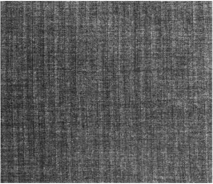
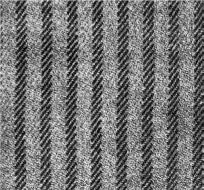
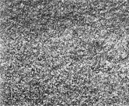
  Figure 3: Sample images

  
  

  f ⁽ z ) = ’

  
  

  f 1

  
  
  
  

  z >  0

  z <  0

  
  
  
  

  From this joint distribution the generic local binary pattern operator is derived. As in the case of basic LBP, it is gained by summing the thresholded differences weighted by powers of two. The LBP P, R operator is defined as

  s - 1

  LBP P , R ( ^xl , y l ) = ^ f ( g s ^{- g}l ).2 s       ⁽¹³⁾

  s = 0

  
  

  5.1. Binary Patterns:

  Consider an image I (x, y) of size m x n and let g l denote the gray level of an arbitrary pixel (x, y), i.e. g l = I (x, y). Moreover, let g s denote the gray value of a sampling point in an evenly spaced circular neighborhood of sampling points and radius R around point (x, y):

  
  

  g s = I ( X s , y s ), s = 0.... S - 1                     (5)

  
  

  x_s = x + R cos(2 ns / S )                       (6)

  y_s = y - R sin (2 ns / S )                      ⁽⁷⁾

  
  

  Similarly for SLBP and LLBP the mathematical representations are given in equations

  sLBP(Xd, yd) = Z s(im - ic )-1

  m = 0

  d-1

  LLBP h ( N , D ) = ^ s ( h m - h d ),2^{( d} - ^{m - 1)} + J [ s ( h m ] - h d ) • 2^{( m} - ^{d - 1)} (15) n = 1                              m = d + 1

  d -1

  LLBP v ( N , D ) = J s ( V m - v ).2^{( d - m - 1)} + J [ s ( v_m ] - V d ).2^{( m - d - 1)} (16)

  m=1

  LLBPm = 4 LLBPh2 + LLBPv2

  
  

  Assuming that the local texture of the image I (x, y) is characterized by the joint distribution of gray values of S+1 (S > 0) pixels:

  
  

  The energy distribution E j (x, y) of the filtered images S j (x, y) is defined as

  
  

  T = t ⁽ g l , g 0 , g 1 ,....g s - 1 )                    ⁽⁸⁾

  Without loss of information, the center pixel value can be subtracted from the neighborhood:

  T = t ⁽ g l , g 0 , g l , g 1 - g l ,-•• g s - 1 ^- g l )        ⁽⁹⁾

  In the next step the joint distribution is approximated by assuming the center pixel to be statistically independent of the differences, which allows for factorization of the distribution:

  T * ⁽ g l ) t ⁽ g 0 ^- g l , g 1 ^- g l ,.... g s - 1 ^- g l )      ⁽¹⁰⁾

  Now the first factor t(g_l) is the intensity distribution over I (x, y). The joint distribution of differences ⁽ g 0 - g l g 1 - g l ,... g s - 1 - g l ) ^can be used ^to model the local texture. Only the signs of the differences are considered:

  t ⁽ f ⁽ g 0 ^- g l ), f ⁽ g 1 ^- g l )•••• f ⁽ g s - 1 ^- g l ))           (11)

  Where f(z) is the thresholding (step) function

  
  

  E y = ZZ i S y ( x >  у )l

  xy

  
  
  
  

  The mean (μ j ) and standard deviation (σ j ) are found as follows:

  
  

  M j

  
  

  ^ j

  
  

  MN

  
  

  E_j ( x , y )

  
  

  MN

  
  

  JJ ^{[( s ]} j ^{( x} , y ) ^- и )²

  xy

  
  
  
  

  5.2. GLCM

  Given an image composed of pixels each with an intensity (a specific gray level), the GLCM is a tabulation of how often dissimilar arrangements of gray levels cooccur in an image. Texture feature calculations employ the GLCM information to provide a variation measure of the intensity at the pixel of interest. Create a GLCM square matrix of size N x N where N is the number of quantization levels. Then, the features such as contrast,

  
  

LLBP algorithm gets the line binary code along with horizontal and vertical direction separately and also its magnitude, which differentiates image intensity changes such as corners and edges as well.

Gray-level co-occurrence matrix (GLCM) is a statistical way of investigative texture that considers the spatial relationship of pixels. It is also recognized as the gray-level spatial dependence matrix. After creating a GLCM by estimating frequent pairs of pixel with precise values in an image, statistical measures are extracted. This is an Ng dimension square matrix, where Ng is the number of gray levels in the image. Element [i, j] of the matrix is generated by counting the number of times a pixel with value i occur as a neighbor to a pixel with value j and then dividing the whole matrix by the total number of such relationship made [3]. Thus each entry is measured as the probability that a pixel with value i will be found nearby to a pixel of value j. The GLCM can be defined as:

P ^Θ ( x , y ) = Pr( I ( p ₁) = x ∧ I ( p ₂) = y ∧ || p ₁ - p ₂|| = d )           (1)

Where P is the probability, p1 and p2 are the positions in the gray scale image I.

Steerable filter is a kind of filter which can filter arbitrary orientation which is produced as a linear combination of the benefits of “basis filter”. The edge at different orientations in an image can be located by splitting the image into orientation sub-bands, Steerable filter allows one to adjust any orientation i.e., to "steer" a filter and to analytically determine the filter output as a function of orientation.

The Steering Constraint is defined as

N

G _θ ( m , n ) = ∑ b_l ( θ ) A_l ( m , n )                (2)

l = 1

Here b l (θ), θ controls the filter orientations and b l is the interpolation function based on the arbitrary orientation. The basis filters A l (m,n) are rotated version of impulse response θ .

N

( m , n ) = ∑ b_l ( θ )( I ( m , n )) A_l ( m , n )          (3)

• l = 1

Generally speaking, the texture image can be seen as a set of basic cyclic primitives characterized by their spatial homogeneity. By applying statistical measures, this information is extracted, and used to capture the related image content as feature vectors. More precisely, we use the mean μ standard deviation σ of the filtered images S j (x, y). And we use contrast, correlation, angular second moment, entropy, difference entropy by considering the presence of homogeneous regions in texture images.Here j=1,2,3,4 represent horizontal orientation, rotation of 45°, vertical orientation, and rotation of -45°, respectively. Given an image I(x, y), its steerable filter decomposition is:

S_j ( x , y ) = ∑∑ I ( x 1, y 1) C_j ( x - x 1, y - y 1)              (4)

• x 1 y 1

• 4.5.    Classifiers

• 4.    5.1. k-NN Classifier

• 4.    5.2. PNN Classifier

Where C j denotes the directional band pass filter at orientations, j=1, 2, 3, 4.

Three different types of classifiers (k-NN, PNN and SVM) are employed in this work for similarity and defect classification of textures. All of them are described in brief in the following three subsections.

In pattern recognition, the k-nearest neighbor (K-NN) algorithm is a technique for classifying objects based on closest training sample in the feature space. K-NN is a type of instance-based learning having a locally approximated function and all computation are postponed until classification. In K-NN, an object is classified based on the majority vote of its neighbors with the object being assigned to the most common class amongst its k nearest neighbors (k is a positive integer, typically small). If the value of k is 1, then the object is just assigned to its nearest neighbor class [3]. The neighbors are taken from a set of correct classification known objects. This is considered as the training set for the algorithm, even if no explicit training step is required.

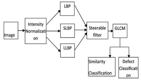
Figure 2: Block diagram of the proposed system

Equations within the structure are selected by Probabilistic Neural Networks using Statistical methods. The PNN is used to categorize the patterns based on learning from instance. It is based on the algorithm of “The Bayes Strategy for Pattern Classification”. Dissimilar rules determine pattern statistics from the training examples. A Probabilistic Neural Network is designed as one containing one input layer, and two hidden layers. When an input is provided, the first layer computes distances from the input vector to the training input vectors and generates a vector whose elements specify the closeness of the input with a training input [13]. The second layer totals these contributions for each class of inputs to produce a vector of probabilities as its net output. Finally, a maximum of these probabilities is picked by the entire transfer function on the output of the second layer and gives an output of a 1 for that class and a 0 for the other classes. The main benefit of PNN is that they are very flexible and with almost no retraining ,new information can be added immediately.

V. TEXTURE CLASSIFICATION ON FABRIC IMAGES:

Some of the sample images used in experiment is provided in fig 3.

In the environment of two-class classification problems, SVM is a learning system that uses an optimal hyperplane to classify sets of feature vectors into two Classes. During the training phase, the hyperplane which has the maximum margin of separation between the two classes is designed as an optimal one [18]. Once the training phase is completed, the test phase begins in which a feature vector not used for training is then classified which fits in to either one of the two classes based on its position with respect to the optimal hyperplane. To compare with a number of classes k larger than two, the one against-one approach is used, i.e., k(k - 1)/2 SVM classifiers being trained on feature vectors from two class memberships only are built, then a test feature vector is linked with the class membership to which it is more frequently associated by the di ff erent SVM classifiers.

correlation, angular second moment, entropy and difference entropy are calculated.

The Contrast feature is calculated as:

N - 1

f ci = S P jk ( j - ^k )²                        (21)

j , k = 0

The Correlation feature is calculated as:

N - 1

fc2= S Pjk j, k=0

(j - y)(k - y)

The Entropy feature is calculated as:

N - 1

fe = S- ln( Pjk) Pjk j, k=0

The Angular Second Moment feature is calculated as:

f w = SS { p ( j , k ) } ²                       (24)

jk

The difference entropy feature is calculated as:

N - 1

fde = -S Px - y (j )log{Px - y (j)}        (25)

j = 0

Where

P jk = Element j, k of the normalized symmetrical GLCM

N= Number of gray levels in the image y= GLCM mean which is calculated as follows

N - 1

y = S ^j Pjk j , k = 0

• <7 ² = intensity variation of all reference pixels which is calculated as follows

N - 1

• ^{7 2} = S P jk ⁽ j ^- y ⁾² j , k = 0

So, the corresponding texture feature vectors of the original image I(x, y) are defined as:

TF 41, _W 2^ 7 3 7 4 , ⁷ 4 , ^f 11, f 21^{, f} _e 1^{, f} Jdevf 12 , f_t 22^{, f} _e 2,L 2 j (2 6)

Thus, a set of feature vectors is obtained as in equation (18). For the experimental analysis we use fabric images of different patterns like star box and dot.

• VI.    EXPERIMENTAL RESULTS

A detailed experimental result analysis is provided in this section. The proposed methodology was implemented using MATLAB 7.10 tool and was evaluated by testing the proposed scheme with different input of fabric texture images. Fig.3 shows the classification result for defect data based on binary patterns. Both binary patterns and GLCM based classification result for defect data is exposed in fig 4.The subsequent figs show the similarity classification results for binary patterns binary patterns and GLCM respectively.

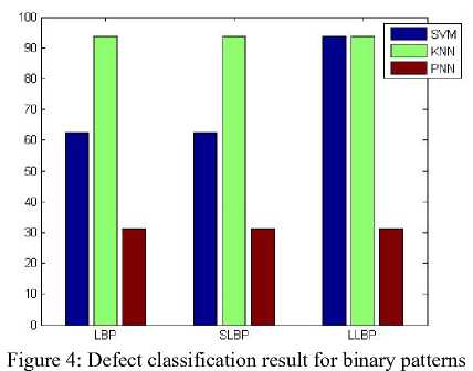
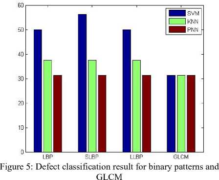
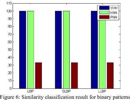
Table of results is provided in the following section. Table 1 reveals the classification rate for defect textures based on the classifiers SVM, K-NN and PNN.

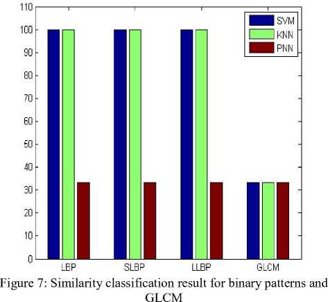
Similarity Classification rate for textures based on the classifiers SVM, K-NN and PNN is shown in table 2. From the first table it is obvious that both SVM and K-NN give exactly the same classification rate for the features used. They give a 100% classification rate for both the binary patterns and for GLCM combined with binary patterns. They give better performance than PNN for defect classification of textures. Table 2 shows that for similarity classification, SVM provides better result for the binary pattern SLBP but much higher result for GLCM combined with binary patterns.K-NN provides better classification rate for GLCM combined with binary patterns than the binary patterns. PNN provides the same classification rate for both binary patterns and GLCM combined binary patterns.

TABLE 1: Defect classification accuracy

Features	Classification accuracy
	SVM	K-NN	PNN
LBP	100	100	33.3333
SLBP	100	100	33.3333
LLBP	100	100	33.3333
GLCM	33.3333	33.3333	33.3333
LBP GLCM	100	100	33.3333
SLBP GLCM	100	100	33.3333
LLBP GLCM	100	100	33.3333

TABLE 2: Similarity classification accuracy

Features	Classification accuracy
	SVM	K-NN	PNN
LBP	50	37.5	31.25
SLBP	56.25	37.5	31.25
LLBP	50	37.5	31.25
GLCM	31.25	31.25	31.25
LBP GLCM	62.5	93.75	31.25
SLBP GLCM	62.5	93.75	31.25
LLBP GLCM	93.75	93.75	31.25

• VII.    CONCLUSION

  In this paper a collective method of binary patterns and steerable filter decomposition is proposed with different binary patterns, GLCM and classification algorithms. The proposed method is tested with the best quality fabric images and two analysis classifications and detection has been sought. From the above results it can be concluded that all the binary patterns and GLCM combined binary patterns proves to be better in measuring defect classification for both SVM and K-NN classifiers. For Similarity classification, both SVM and K-NN provide much higher result for GLCM combined with binary patterns than for binary patterns. It is shown that both SVM and K-NN offer a highest classification rate of 100% and the highest classification rate is 33.3333% for PNN .This can be further extended in the future with the addition of different types of defect textures and also with additional training images.