Clustering Belief Functions using Extended Agglomerative Algorithm

Published Online February 2011 in MECS

• I.    Introduction

  Dempster-Shafer theory (DST) [1,2] is a mathematical tools developed in the 1970s for reasoning under uncertainty. Its strength exists in that it can efficiently cope with imprecise and uncertain information without prior information, thus it is extensively used in many fields, such as information fusion, uncertainty reasoning, pattern recognition, comprehensive diagnosis, etc. The information carrier in DST is belief function.

Corresponding author: Ying Peng.

Combination of belief functions is required for getting a fusion result. And combination is performed just on condition that the belief functions are related to the same event. However, it is usually happened that belief functions related to different events are mixed up, which prevents us from combining them directly. Consequently, it is necessary to distinguish which belief functions are reporting on which event.

Clustering of belief functions can resolve this partition problem. Clustering is an approach that partition data into different clusters. Data in the same cluster are more similar to each other than to members in other clusters. Clustering algorithms such as k-means [3] and hierarchical algorithm [4,5] are the most popular ones for clustering the usual data point. However, different from the usual data point, belief function is uncertain information which cannot be expressed with data point, and the dissimilarity measure between belief functions is more special. Hence, the clustering approaches for data point cannot be used directly to partition belief functions.

So far, the clustering approaches for belief functions can be classified into two main categories: (1) Direct clustering, such as approaches proposed by reference [6], reference [7] and [8]. Approach in reference [6] is based on decomposing of belief functions and Potts spins mean field theory. However, it is complicated and need to set the number of clusters in advance. Compared with this method, approaches in reference [7] and [8] are simpler. Approach in reference [7] is based on k-modes algorithm [9] and belief distance, but it still needs to set the number of clusters, and the results are non-unique due to the selecting of different initialization seed beliefs. Approach presented by reference [8] is based on belief distance and the number of clusters is depended on the threshold values. However, the threshold values are hard to determine. Besides, the approach cannot cope with belief functions with hidden conflict [10]. (2) Indirect clustering, it first needs to transform belief functions into Euclidean characters by TBM [11] or a probabilistic transformation DSmP [12], then clustering algorithms for usual data point can be used. Thereby, approaches in this category are simpler. While the problem is the possible inequality of transformation, and most of the clustering approaches for data point still need to set the number of clusters in advance except for hierarchical algorithm.

This paper is to develop a direct clustering approach which can simultaneously determine the appropriate number of clusters. The rest of the paper is organized as follows. Some definitions in DST are reviewed in Section II. Agglomerative algorithm which is a branch of hierarchical algorithm is presented in Section III. Then, in Section IV, the extended agglomerative algorithm for clustering belief functions is proposed. Three examples are illustrated to validate the effectiveness of the extended agglomerative algorithm in Section V. Finally, we conclude in Section VI.

II. Review of Dst

We list a few definitions necessary in DST to avoid misunderstanding.

Definition 1. (Frame of discernment) The frame of discernment is a finite set of mutually exclusive elements, denoted as Q hereafter.

Definition 2. (Basic belief assignment) A basic belief assignment (bba) is a mapping m from 2 ^Q ^ [0, 1] that satisfies S A _cQ m ( A ) = 1 . The basic belief mass (bbm) m ( A ), A cQ , is the value taken by the bba at A .

When m ( A ) >  0 , A is the focal elements of a bba.

Definition 3. (Dempster’s rule) Let m ₁ and m ₂ be two

bbas defined on frame Q which are derived from two distinct sources. Dempster’s rule of combination two belief functions is given by m = m ₁ ® m 2 , where

S A i n B = A m 1^{( A )} m 2⁽ B )

m ( A ) = •—-—1— k--------, A cQ , A ^ ф ,k ^ 1 (1)

k = V m (A)m (B,) . k is the mass of the i—i Ain Bj =ф 1V l' 2х 1'

combined belief assigned to the emptyset before normalization and called conjunctive conflict for short in this paper.

Definition 4. ( Belief distance ) [13] Let m ₁ and m 2 be two bbas defined on frame Q , the distance between m ₁ and m ₂ is given by

1   ^ ^    ^ ^

d bpa ( m 1 , m 2 ) = 2-m m 1 ,m 1 U ( m 2 , m 2

I ^  ^ \

- 2 ( m ₁, m 2p

where

^ ^

m ₁, m ₂

2 ^N 2 ^N

SS ^m 1^{( A ) m} 2⁽ B j ) i= 1 j= 1

A n B j

A u B j

In

the

following, whenever we use d_BPA or d_BPA ( m ₁, m ₂), we always associate it with belief distance. And d_BPA meets ⁰ — d BPA — ¹ .

• III.    Agglomerative Algorithm

Agglomerative clustering performs in a bottom-up fashion, which initially takes each data points as a cluster and then repeatedly merges clusters until all data points have been merged into a single cluster. The process allows us to decide which level is the most appropriate. Namely we could determine the number of clusters and the clusters by analyzing the hierarchical tree. The agglomerative clustering is more flexible than approaches that need to set the number of clusters first.

Suppose there are n data points. Steps of agglomerative algorithm are described as follows:

Step1 Every data point in a different cluster, and there are n clusters;

Step2 Calculate the dissimilarity between any two clusters;

Step3 Merge two clusters that have smallest dissimilarity, and the number of clusters subtracts 1;

Step4 Repeated step (2) and (3), stop when the number of clusters gets 1.

From the steps above, we can get that the key factor of agglomerative algorithm is the dissimilarity measure between two clusters. The most representative algorithms that measure the dissimilarity between two clusters are single-link [14], complete-link [15], average-link [16], etc.

• IV.    Extended Agglomerative Algorithm For Clustering Belief Functions

The standard agglomerative algorithm which is used for clustering of usual data points shows serious limitations for dealing with belief functions. Firstly, the belief function is uncertain data, so the dissimilarity measure between them is naturally different from that of between the usual data points. Secondly, smallest dissimilarity is not adequate for merging clusters of belief functions because of the possible hidden conflict [10].

To tackle these problems, the agglomerative algorithm is extended from two aspects: ® Belief distance is used to calculate the dissimilarity. ® Consistency test is put forward to control the merging of clusters. If two clusters with smallest dissimilarity are consistent, they can merge, vice versa. Consistency test brings two advantages: one is to avoid the hidden conflict in each cluster, another one benefits the determining the number of clusters. These two issues will be discussed in the following sections.

The dissimilarity measure and the consistency test are presented in section A and B respectively. Section C explains how to determine the number of clusters. The algorithm design is provided in section D .

A. D ss m lar ty Measure

Belief distance defined by (2) is taken as the dissimilarity measure between two belief functions.

The complete-link algorithm is select to measure the dissimilarity between two clusters. Hence, the dissimilarity between two clusters is defined as follows.

d ( r , 5 ) = max ( d BPA ( e ri , e sj ) ) ,1’ € ( 1, L , n,. ) , ^j € ( 1, L , n s )

where d_BPA is the belief distance. n_r is the number of beliefs in cluster r and n_s is the number of beliefs in cluster s . e_ri is the i th belief in the cluster r and e_sj is the j th belief in the cluster s . The range of dissimilarity between clusters is 0 to 1.

It is clear that the dissimilarity between two clusters is the furthest dissimilarity between belief functions in these two clusters. Find two clusters that have smallest dissimilarity by: d ( k , l ) = min ( d ( r , s ) ) . Clusters k and l are called the furthest neighbors. And it is obviously, 0 <  d ( k , l ) < 1.

• B.    Consistency test

In this section, two definitions that are important for consistency test are proposed first. One is leading element in a bba and another one is leading element in a cluster.

Definition 5. (Leading element in a bba) The leading element in a bba is the union of focal elements that get the highest mass except for the frame of discernment Q when m ( Q ) * 1.

When m ( Q ) = 1, the leading element in this bba is Q .

Example below is enumerated to describe the leading elements concretely.

Example 1 Let Q = {c1m2,m3} be a frame of discernment. Suppose four distinct belief functions, defined on Q , are given by m1 ({m}) = 0.8,m, ({m2}) = 0.2 ;

m 2 ( { m } ) = 0.4, m 2 ( { ® 2 } ) = 0.4, m 2 ( { ® з } ) = 0.2 ;

m 3 ( { m ₂, m 3 } ) = 0.8, m 3 ( Q ) = 0.2 ;

m ₄ ( { m } ) = 0.4, m ₄ ( Q ) = 0.6 .

The leading elements of bbas in example 1 are listed in Table I.

TABLE I.

The Leading Elements Of Bbas In Example 1

Bba	{ m J	{ m 2 }	{ m ,}	{ m 4 }
Leading Element	{ m l	I m , « 2 }	{ ® 2, ® з }	{ m l

Definition 6. (Leading element in a cluster) The leading element in a cluster is the intersection of leading elements in bbas that belong to this cluster.

If m ₁ , m ₂ and m ₄ in example 1 are in one cluster C ₁ , the leading element in C 1 is { m } = { m } ^ { m , m ₂} ⁿ { m }.

The definition of consistency test is given as follows.

Definition 7. (Consistency test) If the intersection of leading elements in two clusters is not null, the two clusters are consistent, otherwise, they are inconsistent.

If two clusters are inconsistent, the two clusters should not merge, i.e., they should be in different clusters. In example 1, since { m } n { m ₂, m ₃ } = ф , the third BBA cannot merge with clusters C ₁ .

Example below is used to show that the consistency test is helpful to avoid hidden conflict.

Example 2 Let Q = {m,m2,m3} be a frame of discernment. Suppose three distinct belief functions, defined on Q , are given by m1 ({m, m2}) = 1; m 2 ({m2, m3}) = 1; m 3 ({m, m3}) = 1.

Belief distances between any two of them are equal, and any two of them are consistent, which makes them seem to refer to the same event. However, they should not be partitioned into one cluster, because there is hidden conflict among them, i.e., { m 1 , m 2 } n { m ₂, m ₃ } n { m , m 3 } = ф .

If consistency test is executed, the cluster C 1 = { m , , m ₂} gets the leading element { m ₂ } and the leading element of cluster C ₂ = { m 3 } is { ® 1 , m 3 } . The two leading elements have null intersection ф = { m ₂ } n { m ₁, m 3 } . Consequently, the two clusters C ₁ and C ₂ are inconsistent, which keeps them from merging.

Thereby, it is necessary to implement consistency test before every merging of two furthest neighbors. Just the two furthest neighbors are consistent, they can merge.

• C.    Determining the number of clusters

To determine the number of clusters without any priori information is a difficult problem. Therefore, a majority of approaches for clustering need to set the number of clusters in advance. Although agglomerative algorithm does not need to set the number of clusters in advance, it is still hard to get the appropriate number of clusters after the finishing of clustering.

In the extended algorithm, the inconsistent furthest neighbors cannot merge, and the largest dissimilarity value prevents two clusters from merging. So the problem of determining the number of clusters is easy to resolve with a simple step: reset the dissimilarity between any inconsistent furthest neighbors to 1 which is the largest value of dissimilarity between clusters.

Since the dissimilarities among inconsistent clusters are all 1, it is easy to get the number of clusters from hierarchical tree: when dissimilarities between any two clusters are 1, the clustering is finished and the current number of clusters is the final number of clusters. This is the main advantage of the extend algorithm.

• D.    Algorithm Design

Fig. 1 presents a flow chart of the extended algorithm. And nodes in Fig. 1 are interpreted as follows:

• 1.    Dissimilarity = Dissimilarities between any two clusters are calculated.

• 2.    Fur Nei = Two furthest neighbors are found.

• 3.    Cons Text = Consistency test. Are the two furthest neighbors consistent?

• 4.    Merge = Two furthest neighbors merge, and a new cluster c_l is get.

• 5.    Lead Elem = Leading Element. Get the leading element in the new cluster c_l .

• 6.    Dis 1 = Dissimilarity between two clusters is reset as 1.

• 7.    Update = Update the dissimilarity between two clusters.

• 8.    Finished = Does the clustering finish? If dissimilarities between any two clusters are 1, the clustering finishes.

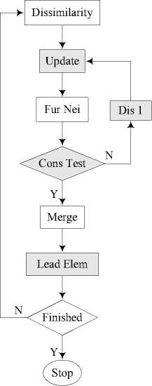
Figure 1. Flowchart of the extended agglomerative algorithm

It is obvious that, except for nodes with shadow, Fig. 1 expresses the standard agglomerative algorithm. And it is the very nodes with shadow make the algorithm capable of coping with clustering belief functions.

V.    Experiments and Discussion

In this section, the validity of the extended algorithm will be validated by the following three typical examples. The first example is composed of Bayesian belief functions which are the simplest type of belief functions. Clustering belief functions of this category is relatively easy. The second example is made up of categorical beliefs, and it contains hidden conflict. Clustering belief functions of this category is some hard. Normal beliefs constitute the third example, which can be taken as the mix of the first two sorts of belief functions, and it is the most common one in real application.

We also give out the clustering results using the approaches in reference [7] and [8] for comparison. The selecting of these two approaches due to their similarities to our extended agglomerative algorithm: they both belong to direct clustering and belief distance is adopted as the dissimilarity measure. For approach in reference [7], we always set the right number of clusters that determined by our extended agglomerative algorithm, and the initialization seed beliefs (ISB) are specified. For approach in reference [8], threshold value p is needed to control clustering process. Hence, we always evaluate appropriate value for p in these three examples.

• A.    Bayesian belief functions

• 1)    Experiment data

Example 3 Let Q = {m,m2,m3} be a frame of discernment. Suppose ten distinct belief functions, defined on Q, are given by e1 : m ({m,}) = 0.5, m ({m2}) = 0.2, m ({m3}) = 0.3 ;

e ₂: m ( { m } ) = 0.0, m ( { m ₂ } ) = 0.9, m ( { m ₃ } ) = 0.1;

e ₃: m ( { m ,} ) = 0.55, m ( { m ₂ } ) = 0.1, m ( { m ₃ } ) = 0.35 ;

e 4 : m ( { m } ) = 0.45, m ( { m ₂ } ) = 0.2, m ( { m 3 } ) = 0.35 ;

e ₅: m ( { m ,} ) = 0.1, m ( { m ₂ } ) = 0.2, m ( { m 3 } ) = 0.7;

e 6 : m ( { m } ) = 0.7, m ( { m ₂ } ) = 0.2, m ( { m 3 } ) = 0.1;

e ₇: m ( { m ,} ) = 0.6, m ( { m ₂ } ) = 0.2, m ( { m 3 } ) = 0.2 ;

e ₈ : m ( { m } ) = 0.2, m ( { m ₂ } ) = 0.5, m ( { m ₃ } ) = 0.3;

e ₉: m ( { m 1 } ) = 0.5, m ( { m ₂ } ) = 0.4, m ( { m 3 } ) = 0.1;

e ₁₀: m ( { m } ) = 0.9, m ( { m 2 } ) = 0.05, m ( { m ₃ } ) = 0.05.

Analyzing the belief functions above, we can get that beliefs e ₁ , e ₃ , e ₄ , e ₆ , e ₇ , e ₉ , e ₁₀ all assign the highest probability to hypothesis m , so it is reasonable to consider that they concern the same event and partition them into one cluster. Beliefs e ₂ and e ₈ are both assign the highest probability to m ₂ , so they are potentially partitioned into the same cluster. Only belief e ₅ gives m 3 the highest probability, which separates itself from other two clusters.

• 2)    Result and discussion

Fig. 2 presents the hierarchical tree of example 3 produced by the extended agglomerative algorithm.

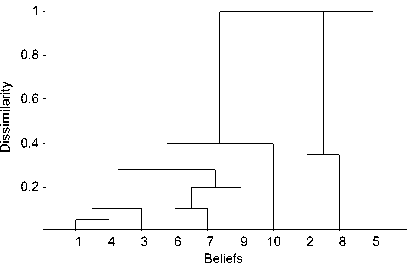
Figure 2. Hierarchical tree of example 3

It is clear that there are three clusters that dissimilarity between any two of them is 1. Therefore, we can easily determine that the number of clusters is 3. The three clusters are also gotten according to hierarchical tree. The clusters and the corresponding leading elements are listed in Table II.

TABLE II.

The Clusters And The Corresponding Leading Elements Of Example 3 Using The Extended Agglomerative Algorithm

Cluster	Leading Element
C 1 = { e1 , e 3 , e 4 , e 6 , e 7 , e 9 , б ю}	{ « }
C 2 = { e 2 , e 8 }	{ « 2 }
C 3 = { e 5 }	{ « 3 }

The clustering results listed in Table II go nicely with the analyses. And we can conclude from Table II that the leading element of each cluster is the event that this cluster concerns.

Table III lists the clustering results of example 3 by using approaches in reference [7] and [8].

TABLE III.

The Clusters Of Example 3 Using Approach In Reference [7] And [8]

Approach	Cluster
[7] ISB= { e 1, e 2, e 3}	C 1 = { e1 , e 3 , e 4 , e 5 , e 8 , e 9 } , C 2 = { e 2 } ,   C 3 = { e 6 , e 7 , e 10 }
[7] ISB= { e 1, e 8, e 5}	C 1 = { e 1 , e 3 , e 4 , e 6 , e 7 , e 9 , e 10 } , C 2 = { e 2 , e 8 } ,   C 3 = { e 5 }
[8] p = 0.35	C 1 ={ e1 , e 3 , e 4 , e 6 , e 7 , e 9 , e 10 } , C 2 = { e 2 , e 8 } ,   C 3 = { e 5 }
[8] p = 0.38	C 1 = { e 1 ,e 3 , e 4 , e 5 , e 7 , e 8 , e 9 } , C 2 ={ e 2 } , C 3 ={ e 6 , e 10 }

Utilizing the approach in reference [7], when ISB are { e ₁, e ₂, e ₃}, we get the wrong clustering result. When ISB= { e ₁, e ₈, e ₅}, we get the right clustering result. Consequently, the approach in reference [7] is unstable, i.e., the selecting of improper ISB can result in wrong clustering.

When threshold value p = 0.35 , approach in reference [8] produces the right clustering. When p changes a little, such as p = 0.38 , beliefs e ₅ and e 8 are in the same cluster with beliefs e ₁ , e ₃ , e ₄ . Obviously, the result is not right. Therefore, the approach in reference [8] is not robust.

• B.    Belief functions with hidden conflict

• 1)    Experiment data

Example 4 Let Q = {«1,«2,L,«8} be a frame of discernment. Suppose nine defined on Q, are given by

e : m ( { « , « ₃ } ) = 1;

e 3 : m ( { ^ 1 , « ₃, « ₈ } ) = 1;

^e 5 : m ( { « 6 } ) = 1;

e 7 : m ( { « 4 , « 5 } ) = 1;

e 9 : m ( { « 2 , « ₃ } ) = 1.

distinct belief functions e2: m({«2,«3}) = 1;

e 4 : m ( { « 4 } ) = 1;

^e 6 : m ( { « 7 , « 6 } ) = 1;

e ₈: m ( { « , « 2 } ) = 1;

Obviously, e ₁ and e ₈ are identical ones, so they should be in the same cluster, we denote it by cluster c . e ₂ and e ₉ should also be in the same cluster because of their sameness, we denoted this cluster as cluster c 2 . For cluster c * , cluster c 2 , and belief e ₃, any two of them are consistent, which usually mistakes us with partitioning them into one cluster. However, there is a hidden conflict existing in these three ones, i.e., { « 1 , « 2 } n { « ₂, « ₃ } п { « , « ₃, « ₈ } = ф . Hence, beliefs e 1 , e ₂ , e ₈ , e ₉ and e ₃ should not be partitioned into one cluster.

Belief e ₅ ensures that hypothesis « 6 is true hypothesis. Belief e ₆ supports hypothesis « ₆ or « ₇ as true hypothesis. The two beliefs have intersection « 6 , therefore, the two beliefs may concern to the same event, and may be in one cluster. Beliefs e ₄ and e ₇ have their intersection « ₄ as true hypothesis, therefore, the two beliefs may be in one cluster.

• 2)    Result and discussion

Fig. 3 presents the hierarchical tree of example 4.

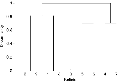
Figure 3. Hierarchical tree of example 4

As shown in Fig. 3, there are four clusters that dissimilarity between any two of them is 1. Consequently, we easily determine that the number of clusters is 4. The four clusters and the corresponding leading elements are listed in Table IV.

TABLE IV.

The Clusters And The Corresponding Leading Elements Of Example 4 Using The Extended Agglomerative Algorithm

Cluster	Leading Element
C 1 = { e 5 , e 6 }	{ ® 6 }
C 2 = { e 4 , e 7 }	{ « 4 }
C 3 = { e 2 , e 9 , e 1 , e 8 }	{ « 2 }
C 4 = { e 3 }	{ « , « 3 }

From the results listed in Table IV, we obtain that beliefs e ₁ , e ₂ , e ₈ , e ₉ and e ₃ are in different clusters, which agrees with the analyses above. The extended agglomerative algorithm gives the reasonable clustering result.

Table V shows the clustering results of example 4 by using approaches in reference [7] and [8].

TABLE V.

The Clusters Of Example 4 Using Approach In Reference [7] And [8]

Approach	Cluster
[7] ISB= { e 1, e 2, e 3, e 4}	C 1 = { e 5 , e 6 , e1 ,e 8 } , C 2 = { e 4 , e 7 } , C з = { e 2 , e 9 } , C 4 = { e 3 }
[7] ISB= { e 1, e 5, e 3, e 4}	C 1 = { e 5 , e 6 } , C 2 = { e 4 , e 7 } , C 3 ={ e 2 , e 9 , e1 , e 8 } , C 4 ={ e 3 }
[8] p = 0.71	C 1 = { e 5 , e 6 } , C 2 = { e 4 , e 7 } , C 3 ={ e 2 , e 9 } , C 4 ={ e1 ,e 8 } C 5 = { e 3 }
[8] p = 0.82	C 1 = { e 4 , e 7 } , C 2 = { e 5 , e 6 } C 3 = { e 1 , e 8 , e 2 , e 9 , e 3 }

For approach in reference [7], when ISB={ e ₁, e ₂, e ₃, e ₄}, we get the wrong clustering result. While when ISB= { e ₁, e ₅, e ₃, e ₄}, the right clustering is obtained.

For approach in reference [8], when p = 0.71, we get five clusters in which C 3 = { e 2 , e 9 } and C 4 = { e_b e 8 } . The result is not right. Beliefs in these two clusters have intersection on true hypothesis, so they concern the same event and should merge into one cluster. When p = 0.82, beliefs e ₁ , e ₂ , e ₈ , e ₉ and e ₃ are in the same cluster. The result is obviously wrong, which reflects that the approach in reference [8] cannot cope with belief functions with hidden conflict.

• C.    Normal belief functions

• 1)    Experiment data

Example 5 Let Q = {®,,®2,l,ю6} be a frame of discernment. Suppose eight distinct belief functions, defined on Q, are given by e1: m ({ю, ю2}) = 0.8, m ({ю3}) = 0.1, m ({®6}) = 0.1;

e ₂: m ( { ® ₂ , ® 3 } ) = 0.85, m ( { ю } ) = 0.15;

e 3 : m ( { ю ю ₃ } ) = 0.6, m ( { ю ₄ } ) = 0.2, m ( { ю ₅ } ) = 0.2 ;

e 4 : m ( { ю ₄ } ) = 0.7, m ( { ю ₂, ю ₅ } ) = 0.2, m ( { ю 3 ,ю ₆ } ) = 0.1;

e ₅: m ( { ю ₄, ю ₅ } ) = 0.8, m ( { ю } ) = 0.2 ;

e ₆: m ( { ю ₄ } ) = 0.8, m ( { ю® 3 } ) = 0.2;

e ₇: m ( { ю ₆ } ) = 0.6, m ( { ю , ю 3 } ) = 0.2, m ( Q ) = 0.2 ;

e ₈: m ( { ю ₃ } ) = 0.8, m ( { ю } ) = 0.2 .

Beliefs e ₄, e ₅ and e ₆ have their intersection ® 4 as the true hypothesis, so they can be divided into the same cluster. Both beliefs e ₁ and e ₂ support ю ₂ as possible true hypothesis, so they may be related to the same events. And so does for beliefs e ₃ and e ₈ . Different from other beliefs, belief e ₇ strongly supports ю ₆ as true hypothesis, so we may consider e ₇ describes a different event.

• 2)    Result and discussion

Fig. 4 presents the hierarchical tree of example 5.

From Fig. 4 we can see that the appropriate number of clusters is 4. The clusters and the corresponding leading elements are given by Table VI.

The clustering result listed in Table VI agrees with the analyses.

Table VII shows the clustering results of example 5 by using approaches in reference [7] and [8].

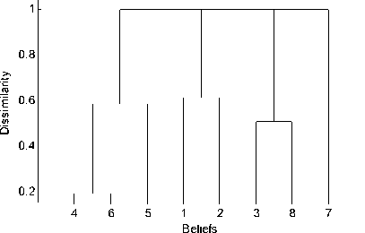
Figure 4. Hierarchical tree of example 5

TABLE VI.

The Clusters And The Corresponding Leading Elements Of Example 5 Using The Extended Agglomerative Algorithm

Cluster	Leading Element
C 1 = { e 4 , e 5 , e 6 }	{ ® 4 i
C 2 = { e 1 , e 2 }	{ ® 2 }
C 3 = { e 3 , e 8 }	{ ® 3 }
C 4 = { e 7 }	{ ® 6 }

TABLE VII.

The Clusters Of Example 5 Using Approach In Reference [7] And [8]

Approach	Cluster
[7] ISB= { e 1, e 2, e 3, e 4}	C 1 = { e 4 , e 5 , e 6 } , C 2 = { e 1 } , C 3 ={ e 2 } , C 4 ={ e 3 , e 7 , e 8 }
[7] ISB= { e 4, e 1, e 3, e 7}	C 1 = { e 4 , e 5 , e 6 } , C 2 = { e 1 , e 2 } , C 3 = { e 3 , e 8 } , C 4 = { e 7 }
[8] p = 0.55	C 1 ={ e 3 , e 4 , e 5 , e 6 } , C 2 ={ e 1 } , C 3 = { e 2 } , C 4 = { e 7 } , C 5 = { e 8 }
[8] p = 0.6	C 1 ={ e 3 , e 4 , e 5 , e 6 } , C 2 ={ e 1 } , C 3 = { e 2 , e 8 } , C 4 = { e 7 }

For approach in reference [7], when ISB= { e ₁, e ₂, e ₃, e ₄}, belief e ₇ is in the same cluster with beliefs e ₃ and e ₈ . Belief e ₇ strongly concerns hypotheses ю ₆ , whilst beliefs e ₃ and e ₈ have their intersection strongly concerns hypothesis ю ₃ . The two hypotheses are incompatible, so the clustering is still not right. When ISB= { e ₄, e ₁, e ₃, e ₇}, the right clustering is gotten.

For approach in reference [8], when p = 0.55 and p = 0.6 , belief e ₃ is always partitioned into the same cluster with beliefs e ₄ , e ₅ and e ₆ . Belief e ₃ strongly concerns hypotheses ю ₁ and ю ₃ , whilst beliefs e ₄ , e ₅

and e ₆ have their intersection strongly concerns hypothesis ω ₄ . The hypotheses that they strongly concern are incompatible, so the clustering is still not right.

In all, above three examples demonstrate the superiority of our extended agglomerative algorithm in below three aspects:

• (1)    The extended agglomerative algorithm can determine the number of clusters by itself. It neither needs to set the number of clusters in advance nor needs to set any threshold value to control it.

• (2)    The extended agglomerative algorithm can avoid hidden conflict.

• (3)    The extended agglomerative algorithm is robust. The clustering result is regardless of the sequence of beliefs or any external control values.

VI. Conclusion

Clustering is necessary when belief functions related to different events are mixed up. However, most of clustering approaches for belief functions need to set the number of clusters in advance. Still, they may be unstable and cannot deal with the belief functions with hidden conflict. In order to solve these problems, an extended agglomerative algorithm is proposed for clustering all types of belief functions that are mixed up. Three typical examples product promising results which indicates the extended agglomerative algorithm is robust and can avoid the hidden conflict. What’s more, the number of clusters is given out by algorithm itself instead of being set in advance. The extended agglomerative algorithm belongs to direct clustering approach, so it avoids the possible inequality transformation, and it is still simple.