Combination of Spatial Filtering and Adaptive Wavelet Thresholding for Image Denoising

Published Online May 2017 in MECS DOI: 10.5815/ijigsp.2017.05.02

Signal processing applications in information and communication technologies are in permanent progress and play a central role in the development of numerical systems of telecommunication and automation; including mobile communications, Radar signals, medical images, satellite images, etc. Nowadays, one of the most important processing adopted in several and sensitive applications is the image processing for which; the employability is widespread in various applications such as recognition systems, meteorological previsions, geographical information systems, etc. The most important performance factors in such images come from their clearness, resolution and compressibility, the fact that the improvement of one of these criteria will intuitively increase the quality of the relating applications.

In this paper, we’ll limit to the denoising operation for opening soon the field to other applications in the future works [1] .

So, estimation of a signal acquired from its transmission channel was for a long time the interest in many research questions for both practical as well as theoretical reasons. Several traditional methods have employed linear methods where the most common choice was the wiener filtering. The challenge then, is, how to recover the original signal from the disturbed data so that the recovered one is nearer the original signal even more clearly and more precise while maintaining the most of its important properties [2] . Therefore, the revolution recorded in multi-resolution analysis from the beginning of the 1980s via the development of the wavelet transforms by GROSSMAN and MORLET (1984) [3-6] has opened a very important field of applications answering to these challenging requests thanks to a certain number of advantages over the traditional approaches. The principal challenges in such approaches consist in determining an optimal threshold value as well as to define a suitable thresholding strategy.

Widely adopted in the wavelet domain, two most widespread thresholding strategies are soft [7] and hard thresholding that differ just by shrinking or maintaining the coefficients above the threshold value [2, 8-12]. So, and whereas each of them is favorable particularly in some cases [11,  13-15], several alternatives were proposed in order to extend these two strategies. Among them we mention: non-negative garrote shrinkage (NGS) [16], firm shrinkage (FS) [16], Trimmed thresholding (TT) [17], Customized thresholding (CT) [2], OLI-Shrink [9], etc.

Although the idea of thresholding is simple and effective, the act of finding a good threshold is never an easy task [11] . Thus, and in order to denoise images generally modelled by (GGD) distribution, a multitude thresholds were set in several research questions including: Universal threshold [12-13, 18-19] , Minimax threshold [12] , SUREShrink [18, 20] , BayesShrink (BS) [11, 18, 21] , Modified BayesSrink (MBS) [21] and Rigorous BayesShrink (RBS) that differs from (BS) by a factor of √2 (T_RBS = √2 T_BS) [22] , NormalShrink [19, 21, 23] , RegularShrink [24] , ProbShrink [18] , and other approaches mainly based on statistic analysis of the wavelet coefficients (like: standard deviation, arithmetic and geometric means) [25] , and so on.

Moreover and in addition to the techniques quoted previously, a multitude of approaches were proposed in the literature based on combinations space filtering/ wavelet schemes. These combinations attending to benefit from advantages of such alternatives include: DWT with histogram equalization as a pre-processing stage [26] , (JBF) using the denoised image as a reference image [27] , (LMMSE) adopting an (OWE) instead of (WT) [28] , (LMMSE) combined with (OWE) and (JBF) [29] , combination of (LPG-CPA) procedure and (JBF) [30] , fusion of bilateral filter (BF) into the wavelet thresholding (WT) to produce a reference image for the (JBF) [31] and so on.

In this paper, and motivated by improving the performances of image denoising via wavelet-based thresholding – that often induces the smoothing effect of the processed image mainly due to the thresholding of all detail sub-bands – we introduce a new alternative that overcomes the shortcoming quoted previously by adopting an interesting combination of spatial and transform domains that allow well benefiting from the advantages of both wavelet thresholding and spatial filtering. So, the acquired image from the transmission channel being degraded by Gaussian noise (with respect to the central limit theorem (CLT)) is decomposed into wavelet coefficients via a two-level 2D-DWT. Then, the finest detail sub-bands (LH1, HL1, HH1) being nearly constituted by only the noise coefficients, an adaptive thresholding is applied to cancel nearly the entire effect of the noise in the processed image. Moreover, the residual noise being mixed within the true coefficients of the coarse detail subbands (LH2, HL2, HH2); an adaptive wiener filtering is adopted to clean those coefficients from the residual noise instead of thresholding them; avoiding so the smoothing effect of the resulting image. Finally, and in order to well preserve the different features of the processed image, a joint bilateral filter (JBF) is performed to the resulting image.

The rest of this paper is organized as follows. In the next section, the wavelet thresholding based image denoising is discussed. Section III describes the new proposed approach with some explanation of its principal components. Simulation results, as well as their suitable comments, are presented in section IV. Finally, a conclusion and perspectives are given at the end of this paper.

• II.    Wavelet Thresholding

Denoising and estimation of functions based on wavelet thresholding lead to simple and powerful algorithms that are often easier to fine-tune than the traditional methods of functional estimation [32]. Multiresolution property and sparse representation of the wavelets are undoubtedly the key factors of an enormous progress recorded in nonlinear thresholding estimations [4]. Moreover, restoring signals and images from their contaminated versions requires strongly taking advantage of the prior knowledge of the whole system and particularly the type of the degradation and its relative information. In this paper, a zero-mean additive Gaussian noise with variance (σ2) is considered. The choice of this degradation has been extensively discussed in the literature, and is principally made with respect to the (CLT) interpreting so, the fact that this kind of noise is found widely occurring in practice [1, 33].

Let us consider a free-noise image F ( x , y ) corrupted by an additive Gaussian noise W ( x , y ) ~ N (0, σ² ) as follows:

G ( x , y ) = F ( x , y ) + W ( x , y )            ⁽¹⁾

From the noisy image G ( x , y ), we try to find an estimate of the original image by removing as much as possible the additive noise W ( x , y ), so that the recovered image being as much as nearer the original one. Therefore, thresholding in multi-resolution expansions and wavelet, in particular, has proven to be very powerful in such problems.

Thus, thresholding in wavelet domain consists principally of three basic steps [1,7,18,32,34] (see Fig. 2): decomposition, thresholding, and reconstruction.

• >    In the first stage, the image of interest is decomposed via an l -level orthogonal wavelet transform leading so to an approximation image from the low pass channel and three directional detail sub-bands (horizontal, vertical and diagonal ±45°) from the high pass channels.

• >    The wavelet transform being orthogonal, the additive Gaussian noise is rightly translated from the spatial to the transform domain   [20] ,  and it is mainly

concentrated in the finest detail sub-bands. So, discrimination of the noise from the true coefficients is done in two main steps.

• •    Threshold computation that allows fixing a level for which the wavelet coefficients below this value are considered to be pure noise. In consequent, this step is often based on the noise level estimation that will be discussed soon in this paper.

• •    Thresholding estimation that consists of choosing an appropriate strategy to be applied to the coefficients above the threshold value. Indeed, the coefficients below the threshold value likely due to noise are often set to zero; while the remaining important coefficients are either maintained without any modifications or shrunk towards zero by some amount. Therefore, two well-known schemes are adopted in the literature: hard and soft thresholding that are depicted in Fig. 1 and defined as follows (for the wavelet coefficients d and the threshold T ):

hard(d) = soft (d) = 0 if <       hard(d) = d         if soft(d) = d - [sign(d) • T] if d < T

d > T d > T

> Finally, the processed coefficients are subjected to an inverse wavelet transform to get the desired image.

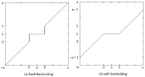
Fig.1. Thresholding Function.

dependent thresholds developed in the literature is one proposed by S. G. Chang et al; namely, BayesShrink (BS) which is an adaptive data-driven threshold for image denoising via wavelet soft-thresholding. It is derived in a Bayesian framework, and the prior used on the wavelet coefficients is the generalized Gaussian distribution (GGD) widely used in image processing applications. It is typically within 5% of the (MSE) of the best soft-thresholding benchmark [11] .

Let us rewrite the model of (1) by its expression in the wavelet domain as:

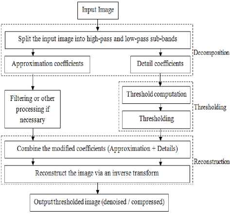
Fig.2. Wavelet Thresholding Algorithm.

Y = X + V                (3)

Where X and Y are the wavelet coefficients of the free-noise and noisy images F and G of the model (1), while V is the wavelet transformed of the additive Gaussian noise W described in (1) which is also Gaussian.

While X and V are mutually independent, the variances: ax , Oy and o² of X , Y and V are related to each other as follows:

Г = r X + r ²              (4)

Moreover, since Y is modeled as zero-mean, Oy can be found empirically by:

r 2 = 4 tft         5

n i , j = 1

Where ( n x n ) is the size of the considered subband.

Thus, from equation (4), the free-noise variance can be derived as follows:

• III.    Proposed Approach

The principal idea behind the realization of this work can be summarized as follows. Although the idea of thresholding in wavelet domain has proven very high performances in resolving many problems related to image restoration from its noisy version, the shrinkage of the wavelet coefficients through all detail sub-bands via this mechanism often leads to considerable losses in fine details of the processed image like edges and the different features inducing so, to smoothing the acquired image. And as a solution, we propose in this paper a new alternative taking advantage of the benefits of both wavelet thresholding and spatial filtering.

• A.    Adaptive Wavelet Thresholding

The simplest thresholding methods work by applying the same threshold to process at least all the wavelet coefficients above a primary resolution level below which no thresholding at all is carried out. However, if the noise in the data is stationary and correlated, then the variance of the wavelet coefficients will depend on the level of the wavelet decomposition but will be constant within each level. Therefore it will be natural to deal differently with the coefficients at each level and to use a level-dependent approach [13]. So, one of the most attractive level er X = -jmax (oY - Г2,0)           (6)

From equations (4 – 6), the most challenging task marking the process of threshold computation via BayesShrink is undoubtedly the noise level estimation. Indeed, D.L. DONOHO and I.M. JOHNSTONE [20] stipulated that is, for practical use, it is important to estimate the noise level (5) from the data rather than to assume that the noise level is known. They believed that is important to use a robust estimator like the median, in case the fine-scale wavelet coefficients contain a small proportion of strong “signals” mixed in with “noise”. In practice, they pioneered the derivation of an estimate from the finest scale empirical wavelet coefficients:

Г = median ({ Y ₇|: Y ₇e subband HH 1 }) / 0.6745   ⁽⁷⁾

Ever since, most of the works established in the field of wavelet-based signal and image thresholding are built upon this estimator thanks to its robustness, nearoptimality, fast and simple computation.

So, the data-driven, sub-band dependent threshold BayesShrink ( BS) is given by [11] :

-max ( Y i , j I) if ^{X 2} ^ ^X Y ) T B ^(X X ^{) -} 1  ,2

^ ст / x_x     otherwise

• B.    Adaptive Wiener Filter ( AWF ):

One of the first methods developed to reduce additive random noise in images is based on wiener filtering which is firstly considered for image restoration in the early 1960s. It is originally derived by minimizing the mean square error between the original and the processed image. One drawback related to the original wiener filter is the blur effect marking the filtered image mainly due to the use of fixed filter throughout the entire image, under the assumption that the characteristics of the signal and noise do not change over the different regions of the image. But, while these assumptions are not really true in practice, it is more reasonable to adapt the processing to the changing characteristics of the image and degradation. One alternative is then, to adaptively design and implement the filter by locally estimating its parameters, leading so to a space-variant wiener filter or adaptive wiener filter [33] .

Therefore, for a particular pixel location ( n 1 , n 2 ), the adaptive wiener-based filtered pixel is given by [33, 35] :

AWF [ I ( n 1 , n 2 ) ] - Ц + ^X--- ^ n - ( I ( n 1 , n 2 ) - ц )      ⁽⁹⁾

СТ

Where the local statistics (mean ц and variance (cr²) are locally estimated from the set К of (N x M ) local neighbourhood of each pixel in the image I . They are estimated as:

Ц ^-

— Y i ( n , n )

1,   2

* n | , n 2 S^

а

-  1 X i ² ( n , n 2 ) - ц¹

mn„ “ ^  ^{1 2}

and ( x n ) is the noise variance.

• C.    Joint Bilateral Filter ( JBF ):

Filtering is one of the most fundamental operations of image processing where the resulting filtered image at a given location is generally a function of the values of the input image in a small neighborhood of the same location. This process is established upon the assumption that images typically vary slowly over space (near pixels are likely to have similar values), and it is, therefore, appropriate to manipulate them together. This assumption is notably violated at edge locations and particularly when low pass filtering is applied, which lead in consequent to blur them. Therefore, many efforts have been devoted to reducing this undesirable effect [36] .

Bilateral filtering is a technique to smooth images while preserving edges by means of a nonlinear combination of nearby image values. It can be traced back to 1995 with the work of Aurich and Weule on nonlinear Gaussian filters and was later rediscovered by

Smith and Brady as part of their SUSAN framework, and Tomasi and Manduchi who gave it its current name [37] . The method is noniterative, local, and simple. It combines gray levels or colors based on both their geometric closeness and their photometric similarity and prefers near values to distant values in both domain and range. It has been used in several contexts such as denoising, texture editing and relighting, tone management, optical-flow estimation and so on [36-37] .

Mathematically, at a particular pixel location ‘ p ’, the bilateral filter (BF) output is given as follows:

Z G x s (I p ^- q I) - G x, ^{( 1} |⁽ p ^{)- 1 (} q ) ) • ^{1 (} q )     (12)

BF ^{[ 1 ( p )] -} q " Z G x s (I p - q | I) - G x , ( Л ( P ) - 1 ( q ) ) q =K ( p )

Where:

G X _S (I p ^- q |I)^{- e}

II p - q | I² 2 x S

[ Gx, (I I ( P ) - I ( q ) ) -

_ 1 1 ( p )- 1 ( q ) 2 2x_r 2

e        ^X

And: К(р) is a spatial neighbourhood of p . While the coefficients ( x_s ) and ( x , ) represent respectively the spatial and range parameters that control and specify the amount of filtering for the image I . In practice, it is shown that in the context of denoising, adapting the range parameter ( x , ) to the estimate of the local noise level yields more satisfying results [37] .

The main drawback of the classic bilateral filter in image denoising is that the edge stopping function G_Cr could not be estimated accurately based on the noisy image. Also, and going from the fact that the waveletbased denoising image proves very high performances in preservation of the most important image features, a some modification is introduced to the original bilateral filter by adopting the wavelet-based denoised image as a reference image instead of the noisy one [27, 38] , leading so to a new variant of the bilateral filter, namely ‘cross bilateral filter’ or ‘joint bilateral filter (JBF)’. In this alternative, the filter smoothes the image to be processed ‘ I ’ while preserving the edges of the reference image ‘ E ’ [37] . So, for a wavelet-based denoised image ‘ E ’ taken as a reference image, the joint bilateral filter (JBF) is described as follows:

Z ^GX_S (I p ^- q ||^)- Gx, ⁽ E ( p ^)- E ⁽ q ) ) • ^{1 (} q )     (14)

^{JBF [ 1 ( p )]-} q " У G x s (I p - ^ D- G x , ( E ( Г ) - E ( q ) ) q =x ( p )

Where the different components are as defined in (10).

• D.    Proposed Algorithm :

As can be clearly drawn from the previous sections, both the spatial filtering and wavelet thresholding prove very high performances in image restoration, making us, so very interesting and highly motivated to take advantage of their efficiencies while keeping all the reserves to take into account the correction of their some relative shortcomings. Indeed, while the wavelet based image denoising has proven very high performances in a wide range of natural images and particularly in case of homogeneous ones, some limits and shortcomings are often present at the resulting images such as artefacts and smoothing effects; mainly due to the thresholding operation and particularly when the processed scenes are relatively dominated by non-homogeneous regions like edges and textures.

In another hand, and opposing to the wavelet theory where the treatments are accomplished in the transform domain, the linear and non-linear filtering (wiener and JBF filtering) processing in the spatial domain have proven to be very powerful in image restoration particularly when the visual criterion is adopted; since the human eye is very sensitive to the overall and the coarse features of the processed scenes more than their intrinsic constitution. However, these spatial approaches also suffer from certain deficiencies and limitations at very low and higher noise levels making them so unfavorable to use them alone in such conditions.

Therefore, and taking advantage of the complementary performances of spatial filtering and wavelet thresholding according to the noise level, we propose within the present paper a new arrangement made by a combination of the advantages of both spatial and wavelet domains; allowing so well denoising the degraded image while preserving the maximum of its details and features. The corresponding algorithm is depicted in Fig. 3 and explained as follows.

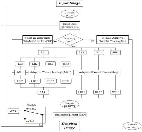
Fig.3. The Proposed Algorithm.

• 1.    First, split the image to be processed into wavelet coefficients via a 2-level (2D-DWT); which results in the first level detail sub-bands (LH1, HL1, and HH1), the second level details (LH2, HL2, and HH2) and the coarse approximation (LL2).

• 2.    From the finest detail sub-band (HH1), compute the estimated level ( ̂ ) of the additive Gaussian noise using the robust median estimator given in equation (7).

• 3.    As well known the efficiency of the adaptive wavelet thresholding (and particularly BayesShrink) at extremely lower noise levels, we adopt this scheme in our algorithm for all estimated values of ( ̂ ) below a some level °п ( °п ≈ 10).

• 4.    Since the detail coefficients of the finest sub-bands (LH1, HL1, and HH1) are very small and are likely due to noise, an adaptive wavelet thresholding (BayesShrink) is applied to these sub-bands in order to cancel approximately the entire effect of the noise in the processed image without affecting its sharpness and its representative details and features.

• 5.    Moreover, the residual noise being mixed within the true coefficients of the coarse detail subbands (LH2, HL2 and HH2) that are more likely due to image details than the additive noise; an adaptive wiener filtering is adopted to clean those coefficients from the residual noise instead of thresholding them avoiding so smoothing the resulting image. The main challenge in this phase is the appropriate choice of the window size containing the neighborhood pixels used in the adaptive wiener filter (AWF). In this paper, we adopted three windows (3x3, 5x5 and 7x7) for lower, medium and higher noise levels respectively. This classification is relative and varies from one image type to another and even from one image to another. For images considered in this paper where their constitution is made by a lot of small homogeneous regions separated by great amount of edges, the three noise intervals are given approximately as follows: lower noise level ( а_п ≈10 to 40) , medium noise level ( °п ≈40 to 65) , higher noise level (   ≈

• 6. (LL2) sub-band being representative of the coarse

• 7.    Finally, and in order to well preserve the different features of the image processed, a joint bilateral filter (JBF) is performed to the resulting image taken as a reference image for the edge preservation, while the smoothed image is altered – according to the noise level estimated – between the noisy image at lower levels below ( а_п ≈30) and adaptive wiener filtered image – with windows as defined in the two last steps – otherwise.

• 8.    At the end of the proposed algorithm, all the processed coefficients resulting from the precedent steps are recombined again to be inverse transformed via a 2- level (2D-IDWT). Hence, the image acquired will be more pleasant by cleaning the additive noise while preserving the most details and important features.

From the next steps, we consider only the cases of ( ̂ ) higher than( О_п ≈ 10).

upper to 65). These values can be drawn from the intuition and the experience of the executor.

approximation of the image from the 2- level decompositions, a small proportion of the noise is probably propagated into this sub-band, and an adaptive wiener filter is applied similarly as done in the previous step. This step allows us to cancel nearly all the residual noise remaining from the last two steps.

• IV.    Simulation Results and Discussions

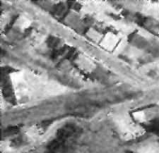
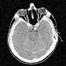
The experiments carried out in this paper are conducted in some relatively non-homogeneous images (512x512) like the satellite image of West-Concord city, a landscape image of a lake and walk-bridge scenes, and a brain MRI image shown in Fig. 4. In our tests, Gaussian noise with different levels (σ = 5, 10, 15, 20, 25, 30, 40, 50, 60, 70) is added to the original scenes to simulate the noisy images. “Symlet” wavelet with eight vanishing moments is employed in the wavelet decomposition and reconstruction steps. (JBF) with parameters ( с₅ = 1.0) and (e r = 0.1) is adopted at the last phase of our algorithm.

Performances of the denoising scheme introduced in this paper are evaluated in terms of (MSE), (PSNR) and correlation coefficient. The first two assessments being quantitative measures give information about the quantity of the noise remaining in the denoised image, and they are formulated for an image of size ( M x N ) by:

MSE

=   ¹   ^Nb [ x ( i , j ) - XX ( i , j ) ] 2

MN и и

( 2.55²

PSNR ( dB ) = 10logJ —

The second measure represented by the correlation coefficient ( ρ ) can be viewed as a qualitative measure; it informs about the similarity and the correlation between the original and the denoised image. It is given by:

p ( % ) = ^{cov (} X ^, XX ) ■ 100% ⁽¹ 7) var ( X ) ■ var ( XL )

Where: X (i,j) and X(_i, j) present the original and the denoised image respectively.

(a) Satellite Image of West-Concord City

(b) Landscape Image of Walk-bridge

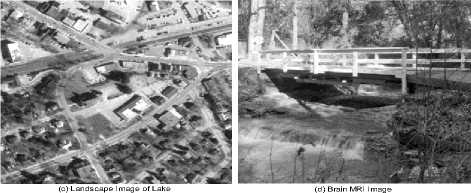
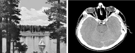
Fig.4. Test images used in the comparison studies of this paper.

To evaluate the performances of the present work, its comparison with the best and recent state-of-the-art approaches relating to the wavelet theory like (BS) with two level decompositions (with analogy to our scheme) and five levels (used as a benchmark comparator) as well as the spatial filtering like the adaptive wiener filter (5x5) is accomplished. The results obtained from the different schemes are reported and compared in Tables 1–5. The better ones among these are highlighted in bold font for each test set.

Table 1. PSNR (dB) results for West-Concord Satellite Image

West-Concord Satellite Image (512x512)
Noise Level ( σ n )	Noisy Signal		Wiener Filter (5 x 5)		BayesShrink (2 levels)		BayesShrink (5 levels)		Proposed
	MSE	PSNR	MSE	PSNR	MSE	PSNR	MSE	PSNR	MSE	PSNR
05	25.06	34.14	110.01	27.72	17.77	35.63	17.76	35.64	17.77	35.63
10	100.23	28.12	121.43	27.29	47.59	31.35	47.49	31.36	47.59	31.35
15	225.51	24.60	138.62	26.71	80.64	29.06	80.23	29.09	67.44	29.84
20	400.91	22.10	159.87	26.09	113.94	27.56	112.69	27.61	89.66	28.61
25	626.42	20.16	183.97	25.48	147.71	26.44	144.83	26.52	117.15	27.44
30	902.04	18.56	210.50	24.90	182.88	25.51	177.22	25.65	146.71	26.47
40	1603.63	16.08	271.33	23.80	257.26	24.03	241.60	24.30	198.72	25.15
50	2505.68	14.14	343.73	22.77	337.16	22.85	303.82	23.30	270.77	23.81
60	3608.17	12.56	428.59	21.81	422.97	21.87	362.28	22.54	315.17	23.14
70	4911.12	11.22	526.12	20.92	516.97	21.00	417.86	21.92	365.61	22.50

From the results of image restoration reported in Tables 1–4, we can clearly notice the effectiveness of our new proposed algorithm in noise-removal from the relatively non-homogeneous images by providing very interesting (MSE) and (PSNR) performances compared to those of the best literature such the adaptive wiener filter and BayesShrink and exceeding them most of the time. Indeed, even if the application of BayesShrink – with high decomposition levels – in that process provides the best results at lower noise levels, our approach remains very competitive which is within 0.05 dB of (PSNR) and 0.8% of the (MSE) of the best adaptive wavelet thresholding benchmark (BayesShrink with 5 levels) and outperforms it again interestingly in terms of the implementation cost and complexity the fact that our scheme requires only two decompositions for all the denoising process opposing to the benchmarked-BayesShrink that adopts generally more than three decompositions. Also, at these lower noise levels, our scheme is built solely upon 2-level BayesShrink for which the (MSE) and (PSNR) results of the denoised images show that this approach is well adequate for weak noise-levels the fact that the computation of the value of the threshold and consequently the shrinkage rate of the coefficients often depends on the level of the additive noise, from where the effect of shrinkage will be appreciably weak on these levels.

Table 2. PSNR (dB) results for Walk-bridge Image

Walk-bridge image (512x512)
Noise Level ( σ n )	Noisy Signal		Wiener Filter (5 x 5)		BayesShrink (2 levels)		BayesShrink (5 levels)		Proposed
	MSE	PSNR	MSE	PSNR	MSE	PSNR	MSE	PSNR	MSE	PSNR
05	25.06	34.14	142.23	26.60	25.45	34.07	25.44	34.08	25.45	34.07
10	100.23	28.12	154.25	26.25	68.35	29.78	68.14	29.80	68.35	29.78
15	225.51	24.60	172.02	25.78	113.53	27.58	112.61	27.61	102.91	28.01
20	400.91	22.10	193.58	25.26	157.91	26.15	155.39	26.22	130.44	26.98
25	626.42	20.16	217.87	24.75	199.61	25.13	194.17	25.25	160.66	26.07
30	902.04	18.58	244.68	24.25	238.29	24.36	228.24	24.55	198.33	25.16
40	1603.63	16.08	306.38	23.27	312.60	23.18	287.12	23.55	252.99	24.10
50	2505.67	14.14	379.48	22.34	390.00	22.22	339.30	22.82	311.40	23.20
60	3608.17	12.56	464.61	21.46	473.21	21.38	385.58	22.27	353.54	22.65
70	4911.12	11.22	562.33	20.63	564.61	20.61	427.90	21.82	401.81	22.09

Table 3. PSNR (dB) results for Lake Image

Lake image (512x512)
Noise Level ( σ n )	Noisy Signal		Wiener Filter (5 x 5)		BayesShrink (2 levels)		BayesShrink (5 levels)		Proposed
	MSE	PSNR	MSE	PSNR	MSE	PSNR	MSE	PSNR	MSE	PSNR
05	25.06	34.14	56.35	30.62	21.91	34.72	21.86	34.73	21.91	34.72
10	100.23	28.12	67.78	29.82	47.35	31.38	46.92	31.42	47.35	31.38
15	225.51	24.60	84.72	28.85	74.74	29.40	73.22	29.48	58.47	30.46
20	400.91	22.10	105.28	27.91	101.07	28.08	97.30	28.25	78.37	29.19
25	626.42	20.16	128.43	27.04	127.74	27.07	120.31	27.33	103.29	27.99
30	902.04	18.58	154.11	26.25	155.88	26.20	143.09	26.57	134.04	26.86
40	1603.63	16.08	213.96	24.83	217.35	24.76	187.66	25.40	165.10	25.95
50	2505.67	14.14	285.66	23.57	287.26	23.55	230.67	24.50	202.52	25.07
60	3608.17	12.56	369.60	22.45	365.57	22.50	271.88	23.79	245.40	24.23
70	4911.12	11.22	466.34	21.44	453.15	21.57	310.63	23.21	291.71	23.48

Table 4. PSNR (dB) results for Brain MR Image

Brain MR Image (512x512)
Noise Level ( σ n )	Noisy Signal		Wiener Filter (5 x 5)		BayesShrink (2 levels)		BayesShrink (5 levels)		Proposed
	MSE	PSNR	MSE	PSNR	MSE	PSNR	MSE	PSNR	MSE	PSNR
05	25.06	34.14	21.84	34.74	11.72	37.44	11.65	37.47	11.72	37.44
10	100.23	28.12	30.94	33.23	31.09	33.21	30.50	33.29	21.43	34.82
15	225.51	24.60	45.11	31.59	54.11	30.80	52.05	30.97	49.70	33.24
20	400.91	22.10	63.36	30.11	80.44	29.08	75.47	29.35	42.91	31.80
25	626.42	20.16	84.94	28.84	108.54	27.78	98.86	28.18	58.03	30.49
30	902.04	18.58	109.75	27.73	137.60	26.74	121.06	27.30	76.31	29.30
40	1603.63	16.08	170.06	25.82	199.38	25.13	161.96	26.04	103.79	27.97
50	2505.67	14.14	244.89	24.24	270.06	23.82	201.12	25.10	138.02	26.73
60	3608.17	12.56	333.36	22.90	353.88	22.64	242.61	24.28	177.57	25.64
70	4911.12	11.22	434.85	21.75	450.66	21.59	285.83	23.57	222.24	24.66

In another hand, and as expected theoretically for medium and higher noise levels, the new proposed approach clearly marked the best results compared to the best literature of wavelet thresholding and spatial filtering. Indeed, and compared to (BS) with the same number of decompositions, we notice well that our approach generally exceeds it for all the levels of the additive noise by an improvement reaching or exceeding the 1dB of (PSNR). This efficiency is still retained in comparison with the benchmarked (BS) by an enhancement of about 0.27 ~ 1 dB of (PSNR) for the West-Concord, lake and walk-bridge images, for reaching and even exceeding the 2 dB for the brain image. Our approach also outperforms notably the adaptive wiener filter by an improvement of nearly 1dB of (PSNR) and 10% of (MSE) along all the noise levels and considerably exceeding them sometimes.

Furthermore, in addition to the numerical criteria of (MSE) and (PSNR) used above, a qualitative evaluation via the correlation coefficient (ρ) is also set in this paper in order to study the similarity and the correlation of the restored image to the original free-noise one. The relating results are well summarized in Table 5. Therefore, the obtained results show that our proposed scheme proves better performances in terms of closeness and similarity of the recovered image to the noise-free one thanks to the preservation of its maximum descriptive and sharp details like edges and the different features. Indeed, our new proposed algorithm succeed to bring a notable enhancement of the noisy image by an improvement reaching the 30% of its initial state and even exceeding it for attaining sometimes the 50% at higher noise levels. Moreover, our algorithm also outperforms the other restoration methods like the benchmarked (BS) by an amount of approximately 0.1% ~ 0.5%, wiener filter and 2-level (BS) by nearly: 0.1% ~ 1.5% for brain MRI image, 0.2% ~ 2% for lake landscape image, reaching and sometimes exceeding the 2% for walk-bridge landscape image and West-Concord satellite image.

Table 5. Correlation (%) results for all the test images

Noise Level ( σ n )	West-Concord Satellite Image (512x512)					Walk-bridge image (512 x 512)
	Noisy Signal	Wiener Filter	BayesShrink		Proposed	Noisy Signal	Wiener Filter	BayesShrink		Proposed
			(2levs)	(5levs)				(2levs)	(5levs)
05	99.59	98.25	99.70	99.70	99.70	99.58	97.60	99.57	99.57	99.57
10	98.37	98.01	99.20	99.21	99.20	98.34	97.39	98.83	98.84	98.83
15	96.45	97.74	98.65	98.66	98.88	96.38	97.07	98.06	98.07	98.25
20	93.93	97.36	98.09	98.11	98.50	93.82	96.68	97.29	97.33	97.77
25	90.97	96.93	97.52	97.56	98.03	90.82	96.24	96.57	96.65	97.24
30	87.70	96.45	96.93	97.01	97.54	87.51	95.76	95.90	96.05	96.58
40	80.75	94.59	95.69	95.90	96.64	80.49	94.67	94.62	95.01	95.62
50	73.86	94.13	94.38	94.81	95.43	73.53	93.41	93.32	94.07	94.58
60	67.43	92.71	93.00	93.78	94.63	67.07	92.00	91.96	93.23	93.82
70	61.63	91.14	91.55	92.80	93.73	61.27	90.44	90.52	92.46	92.97
Noise Level ( σ n )	Lake image (512 x 512)					Brain MR Image (512x512)
	Noisy Signal	Wiener Filter	BayesShrink		Proposed	Noisy Signal	Wiener Filter	BayesShrink		Proposed
			(2levs)	(5levs)				(2levs)	(5levs)
05	99.71	99.36	99.75	99.75	99.75	99.86	99.88	99.93	99.93	99.93
10	98.85	99.22	99.44	99.45	99.44	99.43	99.83	99.82	99.83	99.89
15	97.48	99.02	99.13	99.15	99.32	98.73	99.74	99.69	99.70	99.84
20	95.64	98.77	98.82	98.86	99.08	97.78	99.64	99.54	99.57	99.78
25	93.42	98.50	98.51	98.59	98.79	96.59	99.51	99.38	99.43	99.71
30	90.92	98.19	98.18	98.32	98.43	95.19	99.37	99.21	99.30	99.63
40	85.34	97.49	97.47	97.79	98.07	91.90	99.02	98.86	99.07	99.46
50	79.48	96.65	96.67	97.28	97.62	88.12	98.59	98.45	98.84	99.29
60	73.73	95.69	95.79	96.79	97.11	84.09	98.08	97.98	98.60	99.03
70	68.32	94.62	94.84	96.32	96.56	79.96	97.51	97.44	98.35	98.82

Noisy Image

Wiener Filtred Image

5-levels Bayes Shrinked Image                      Proposed Denoising Approach

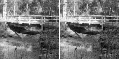
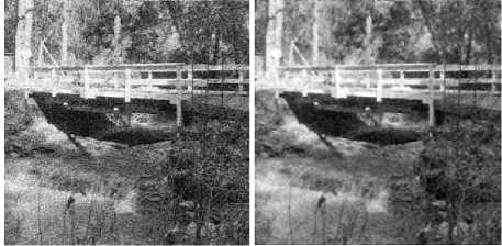
Fig.5. Denoising results of Walk-bridge landscape image at ( σ n =40).

Noisy Image

5-levels Bayes Shrinked Image

Wiener Filtred Image

Proposed Denoising Approach

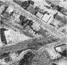
Noisy Image

Wiener Filtred Image

roposed Denoising Approach

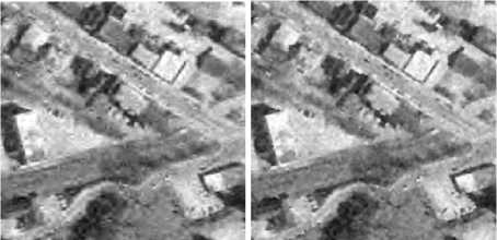
Fig.6. Denoising results of West-Concord Satellite image at ( σ n =40).

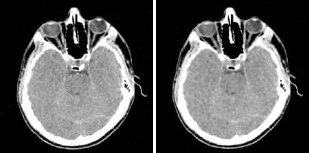
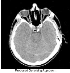
Fig.7. Denoising results of Brain MRI image at ( σ n =40).

Visually, however, the proposed denoising method has proven to perform better in image restoration of relatively non-homogeneous scenes by recovering the different fine details constituting generally the basic building of those classes. Therefore, Fig. 5 shows clearly the superior performances of the proposed approach in application to the walk-bridge landscape image which results in visually more pleasant images than the other methods. Another visual example is depicted in Fig. 6, which illustrates part of the West-Concord satellite image. Again, we can see that in addition to the best recovering of the smooth regions, the details over the contours, ridges and edge points are also well and better recovered using our hybrid scheme. Note also that according to Fig.5–7, (BS) produces more visible artifacts around strong edges, while the adaptive wiener filter smoothes them. And in order to show the contribution of our new proposed algorithm in overcoming these shortcomings, Fig. 7 depicts another example with the Brain (MRI) image (<гп = 40) where the artefacts often introduced due to the thresholding processes around edges are well cancelled using our approach. So, the proposed method provides very high performances in preserving edges and fine details while removing noise. These improvements are reached thanks to the effective exploitation of the advantages of spatial filtering in collaboration with the adaptive wavelet thresholding, which assign it the effectiveness character by preserving the edges and the various important details of the image in the best way during the noise removal process.

• V.    Conclusion

In this paper, a simple and effective approach for image restoration of relatively non-homogeneous images combining the advantages of spatial filtering and adaptive wavelet thresholding is presented. Thus, this hybrid approach is tested successfully on several relatively non-homogeneous images where preservation of edges is the greatest challenge during their processing, and consequently, it is well recommended as a best qualified and effective model for denoising of such kinds of images. The key factors of the effectiveness of this approach can be summarized in two principal points. The first being the restriction of the application of the adaptive wavelet thresholding – adopting only two level decompositions – to just the finest detail sub-bands likely due to the additive noise, allowing so to maximally clean the noise effect from the degraded image while minimize the high computational and implementation costs often due to the multi-decompositions of the conventional denoising approaches. The second point of this approach is the application of an appropriate spatial filter for the remaining sub-bands, allowing so to remove and cancel the residual noise of the first stage avoiding so the smoothing effect generally accompanying the thresholding mechanism, and thus guarantee a maximum edge and details preservation of the processed image. So, our new proposed restoration algorithm is highly recommended when either visual pleasant, quantitative improvement or computation/implementation costs are desired. It is also possible to improve the performances of this approach by generalizing it to other flexible multiresolution transforms ensuring the best descriptions of the different features and descriptive details of the images.