Combined appetency and upselling prediction scheme in telecommunication sector using support vector machines

Published Online June 2019 in MECS DOI: 10.5815/ijmecs.2019.06.01

The rapidly mounting issues in the telecommunication sector today are growth and competition. Understanding customers is vital in the extremely competitive telecom industry. In view of this, Customer Relationship Management (CRM) has become a critical and comprehensive strategy for managing and interacting with customers to improve customer retention and also to attract potential customers.

Guo-en et al. [1] estimated that the average churn rate for the mobile telecommunication is 2.2% per month. Telecom companies spend hugely in acquiring new customers every year and so not only does a company loose future revenue when a customer switch provider (churn) but also the resources spent in acquiring the customer. To combat this challenge, researchers and industries had to advent to a more sophisticated data mining techniques rather than the traditional methods. The knowledge discovery in data (KDD) technology has made it possible to derive more brilliant and advanced knowledge from large data collections. KDD obtain knowledge by extracting patterns from data. The patterns generated could be used to help companies foresee the likelihood of a customer to churn and therefore develop better retention measures [2, 3].

In Customer Churn Predictions (CCP), customers are categorized into two sets of classification behaviors known as churn and Non-churn. A customer is categorized as a churner when they switch from one service provider to the other. Non-churn customers contrarily are loyal customers who do not switch provider and may buy new product or services (appetency), and/or buy upgrades or add-ons (up-selling). Appetency and upselling are important strategies in customer retention and when done correctly can benefit telecom companies in the following: (i) Generate more revenue, (ii) bring in new customers, (iii) help retain customers longer, (iv) get customers to spend more, (v) give customers a fair value of what they deserve.

However, appetency and up-selling have not widely been researched in the telecommunication sector. To bridge this research gaps, this study aims to develop an accurate and comprehensible prediction scheme for appetency and up-selling predictions using machine learning algorithm via support vector machine (SVM). SVM algorithm is implemented in this study because it has been proven to be an effective classification approach for CCP [4] compared with Artificial Neural Network

(ANN), decision tree, logic regression and Naïve Bayesian classifiers.

• II.    Related Works

Since customer churn is an important issue, several authors have been conducting investigations and proposing methods for churn prediction. Ammar et al. [5] presented a meta-heuristic based CCP approach using a hybridized form of firefly algorithm as the classifier. This approach compares every firefly with every other firefly to identify which one has the highest light intensity. The hybridized firefly algorithm provides effective and faster results. Bloemer et al. [6] suggested that a greater degree of customer satisfaction enhance the general performance of a company in the highly competitive telecom industry. Customer satisfaction has in recent years been the focus of most companies thereby giving birth to various machine learning techniques being applied for CCP. Amin et al. [2] proposed a rough set theory (RST) CCP method utilizing Exhaustive Algorithm (EA), Genetic Algorithm (GA), Covering Algorithm (CA), and the LEM2 Algorithm. The results indicated RST based on GA as the overall best performed method for knowledge extraction from publicly available telecom dataset. Caigny et al. [7] proposed a new hybrid algorithm, the logit leaf model (LLM) for better data classification. The proposed algorithm consists of two stages: a segmental phase where customer segments are identified using decision rules and a prediction phase where a model is created for every leaf of the tree. In this approach, LLM outperformed its building blocks i.e. logistic regression and decision tree with a significant predictive score.

• III.    Methodology

In this section, the appetency and upselling classification scheme based on SVM is presented. We proceed to explain the theory behind SVM and the various SVM kernel functions that are adopted in this work. Ultimately, the basis of SVM posterior probability and its application in the proposed prediction scheme are detailed.

• A.    Support vector machine (SVM)

Consider a classification task, in which data is separated into training and testing sets. Each instance in the training set contains one class label and several corresponding features or attributes. In SVM, the goal is to use the training data to produce a model which can predict the class label of each independent instance in the testing data based on their features or attributes. Let (xi, У!), i = 1,—, l be a training data set, where x, e Rn and y( e{1,-1}1 . n is the number of attributes of each input x , y is the class label of input x and l is the number of training points  [12]. Supposing the data is linearly separable, a hyperplane of the form described in (1) can be used to separate the two classes.

w . x + b = 0                    (1)

where w is a weight vector, x is input vector and b is bias [13] . The support vectors are the data points in the training set closest to the hyperplane. SVM finds the optimal hyperplane such that the separation between that hyperplane and the support vectors is maximized. Eliminating any or all of the support vectors would change the position of the optimal separating hyperplane, since they are the critical elements of the training set. In order to apply SVM to classify each instance in the testing data, the solution of the following optimization problem is required:

l

C П

= 1

1 _T min — w w + w , ь , 5 2

Subject to

y,( wT ф( x)+ь )^1 - 5             (2)

where 5 ^ 0 . ф is a function which maps the training vectors x into a higher dimensional space such that SVM finds a linear separating hyper plane with the maximal margin between the classes in this space. C >  0 is a regularization parameter of the error term [14] . 5 is a positive slack variable which is applied to enable SVM handle data that is not completely linearly separable.

• B.    Kernel Functions

  Instead of using the original input attributes x in SVM, some features ф ( x_i ) may rather be applied to get SVMs to learn in the high dimensional feature space [15] . Considering a feature mapping φ , the corresponding Kernel can be defined mathematically as

  
  

  P ( s j ) = 1 n ,

  
  

  max

  sj < yi =—1 max Si < Sj < max

  y i =— 1            y i =+ 1

  max

  ^Sj >  y i =+ 1

  
  
  
  

  K ( x i , x j ) = ^ ( x ) T p ( x j )

  
  
  
  

K (x,, x}) could be easily solved by determining ф (x,) and ф (Xj ) computing their inner product without needing to identify or represent the vectors ф(хг) explicitly. K (x,, Xj ) is a measure of the similarity between ф (x,) and ф (x,)  , and consequently between the two independent attributes x andx . SVM makes predictions using a linear combination of kernel basis functions. The kernel defined by the function in (3) is known as the linear kernel and can work perfectly well for linearly separable data. On the other hand, non-linear kernels are required when data is not fully linearly separable. Therefore, we use a non-linear SVM kernel, the polynomial kernel, in addition to the linear kernel for classification purposes in this paper. The polynomial kernel is one of the quintessential non-linear kernels and can be defined by

K ( x , x j ) = ( y x' T x j + r ) , y >  0

where γ, r and d are the parameters defining the kernel’s behavior [16] .

• C.    Posterior probability

Posterior probability is a theory in Bayesian statistics used to determine the probability of an event given the knowledge of occurrence of other events that bear on it. It can be defined as the conditional probability of a random event or an uncertain proposition after considering key background information on randomly observed data [17] . Contextually, the term ‘posterior’ relates to a hypothesis of what can be ascertained through an understanding of how certain things occur, taking into account the relevant evidence. Posterior probability may be applied in classification to indicate the uncertainty of placing an observation in a particular class.

In machine learning, transforming class membership values into posterior probabilities allow for comparison and post-processing [18] . For SVM, the posterior probability is a function of the score P ( s ) that an instance j is in class y = { - 1,1 } . In the case of linearly separable data sets, the posterior probability is evaluated according to the step function (5).

where s, is the score of the instance j; +1 and ? denote the j positive and negative classes, respectively; n is the prior probability that an instance is in the positive class. The following sigmoid function computes the posterior probabilities for linearly inseparable data classes:

P (Sj ) =------T------\ x 77   1 + exp (As; + B)

where the parameters A and B are the slope and intercept parameters, respectively [19] .

• D.    The Prediction Scheme

In customer churn prediction, posterior probability using SVM is an indication of the probability of a customer to churn or remain with a service provider such as a mobile network operator. For customers who do not churn, they may want to buy new products or an upgrade. In other words, for a randomly selected customer, there could be a conditional probability of buying a new product or an upgrade only if he remains with the network provider. In this paper, a data set of customers’ attributes and class labels (churn or non-churn) is used to train SVM algorithms so that it can make customer churn predictions based on randomly distributed testing data. The class membership scores that SVM evaluates to classify customers are subsequently transformed into posterior probabilities to make appetency and up-selling predictions. Our proposed prediction scheme leverages the posterior probability of belonging to a non-churn class to determine the level of a customer satisfaction. We postulate that the posterior probability is an indication of the level of customer’s satisfaction with a mobile network provider’s services. Customer satisfaction level is derived from a satisfaction score, which is calculated from the posterior probability of belonging to the non-churn class. We obtain the customer satisfaction score c of a customer j as c = p * P ( s_; ) , where P ( s _y) is posterior probability of customer j being in the non-churn class based on its membership score s and β=10 is a score normalization factor. Based on a customer satisfaction level, we can make future inferences about his appetency and up-selling behavior as shown in Table 1.

Table 1. Customer satisfaction scores and attributions

Customer Satisfaction Score	Customer Satisfaction Level	Potential Customer Attribute
8-10	Very Satisfied	•    Remain •    Upgrade •    Buy new product
6-7.99	Satisfied	•    Remain •    Upgrade
4-5.99	Okay	•    Remain
2-3.99	Not Satisfied	Switch but may return
0-1.99	Very Dissatisfied	Switch and may never return

• IV.    Empirical Analysis

• A.    Data preparation and feature selection

  Acquiring actual dataset from telecom industries can be a great challenge due to customer privacy. Nonetheless, there are publicly available datasets for data analysis. Access to the dataset used in this study can be found at the University of California, Irvine, telecom dataset, UCI repository [20]. With 3333 instances consisting of 2850 (85.5%) non-churn (NC) and 483 (14.49%) churn (C) customers, this dataset is considered ideal for modeling. A series of experiments based on the proposed prediction framework is conducted out using MATLAB toolkit. Fig. 1 is a visual presentation of the proposed framework.

Table 2. Attribute description

Attribute	Description
account length	No. of days a customer has been using the service
Intl_Plan	If a customer has international plan or not
VMail_Plan	If a customer has voice mail plan or not
VMail_Msg	Number of voice mail messages
Day_Mins	Daytime minutes used by the customer
Day_Calls	Daytime calls used by the customer
Eve_Mins	Evening time minutes used by the customer
Eve_ Calls	Evening time calls used by the customer
Night_Mins	Night time minutes used by the customer
Night_calls	Night time calls used by the customer
Intl_Mins	Minutes of calls made whiles abroad
Intl_Calls	Calls made whiles abroad
CustSer_calls	Number of calls made to customer care center
Churn?	1 for churners and 0 for non-churners

To reduce computational cost, feature selection has become an important process in knowledge discovery [21, 22]. There are 21 attributes in the dataset used in this study. However, not all attributes in a dataset are suitable for modeling [23]. Some attributes are unique and contain no predictive value, therefore they cannot be used in modeling. In this dataset, the “state, area code, phone number” presents customer information, and “the four charge attributes” have been eliminated since they do not contain relevant information for prediction [4]. Categorical values are normalized by converting ‘yes’ or ‘no’ and ‘true’ or ‘false’ into 1s and 0s. 3. Oversampling was performed on the training set by duplicating the minority class (churn) to obtain almost equal number of minority to majority class. Table 2 describes the influential attributes used in the modeling process.

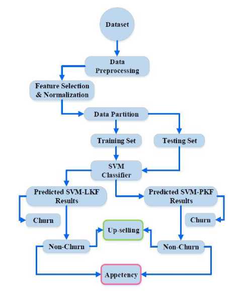
Fig. 1. Visualization of proposed prediction framework.

• B.    Data Partition

In other to evaluate the performance of a trained prediction model, a different set of data other than the one it was trained on is required for validating. This new set of data is the validation set. Validation ensures the model remembers the instances it was trained on and to perform well on unseen new instances [24]. In this paper, we presented a random sampling sizes of (70 – 80) % training set to (30 - 20) % test set for finding how they impact the classifier’s decision. Table 3 describes the training and test datasets after partitioning.

Table 3. Distribution of training and test set

Training set (%)	Observations	Test set (%)	Observations
80	2667	20	666
77	2567	23	766
75	2500	25	833
72	2400	28	933
70	2333	30	1000

• V.    Results and Discussions

This section explores the performance of the proposed study and evaluates the results of the different kernel functions through standard evaluation measures. In subsection A, the churn predictions accuracy results of both models are discussed. Subsection B presents the predicted results of the number of likely up-selling and appetency customers. The least minimum predicted errors of both kernels in subsection C.

• A.    Churn Accuracy Prediction

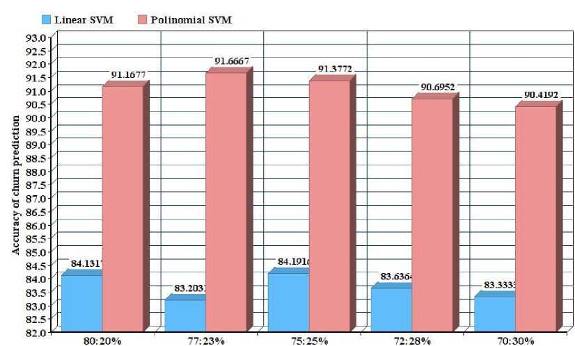
In this section, the accuracy results of both kernels in terms of correctly predicted churn and non-churn customers are evaluated. It is observed that both proposed models exhibit different performance using different sample sizes. The linear kernel however, has the lowest accuracy of 83.203% using a sample size of 77:23%. Fig. 2 demonstrate that polynomial kernel function obtained the best prediction accuracy of 91.67% using a sample size of 77:23% and an overall accuracy of (above 90%) as compared to linear kernel function which predicted an accuracy of 84.19% using a sample size of 75:25% and an overall accuracy of (above 83%).

Sample sizes

Fig.2. Accuracy of churn prediction

• B.    Number of likely up-sell and appetency customers

In general, the number of predicted appetency and up-sell customers increases when the sample size is reduced because there is an increase in non-churn predictions. However, for linear kernel, a change in sample size from (77:23 to 75:25) % slightly reduces the number of predicted appetency customers. Using a sample size of 70:30, the linear kernel predicted the maximum number of upselling (988 customers) and appetency (817 customers) as shown in tables 4 and 5.

Table 4. No. of likely up-sell customers

Sample sizes (%)	Linear	Polynomial
80:20	627	572
77:23	767	654
75:25	786	715
72:28	925	803
70:30	988	863

Table 5. No. of likely appetency customers

Sample sizes (%)	Linear	Polynomial
80:20	510	522
77:23	690	598
75:25	677	651
72:28	764	735
70:30	817	793

C. Minimum error (ME)

This section discusses the results of the ME of the prediction models. These errors are generated when a churner is rather predicted as a non-churner. A wrong non-churn prediction will lead to an error in appetency and up-selling predictions. Table 6 reflects the comparison of predicted errors of our proposed models in up-selling and appetency using different sample sizes. It can be seen that the polynomial kernel predicted the least ME value in up-selling of 0.0587 using a sample size of 75:25% compared with the linear kernel with least ME value of 0.1388 using a sample size of 80:20% in upselling. Also in appetency, polynomial kernel predicted the least ME value of 0.0364 using a sample size of 80:20%. The linear kernel on, the other hand, predicted a least ME value of 0.0765 using a sample size of 80:20%. In general, polynomial kernel function predicted the least ME across all sample size.

Table 6. Me of linear and polynomial kernel functions

	Up-selling		Appetency
Sample sizes	Linear	Polynomial	Linear	Polynomial
80:20	0.1388	0.0594	0.0765	0.0364
77:23	0.1669	0.0596	0.142	0.0385
75:25	0.1412	0.0587	0.099	0.0369
72:28	0.16	0.0648	0.127	0.0422
70:30	0.1609	0.0718	0.1248	0.0492

• VI.    Conclusion

This paper presents a novel up-selling and appetency prediction scheme using SVM algorithm with two different kernel functions. After evaluation of the results, it was observed that polynomial kernel function had the highest accuracies (above 91%) for the first three sample size (i.e. 80:20, 77:23, 75:25) % in predicting both churners and non-churners compared with the linear kernel function. The proposed scheme speculates using the posterior probability of customers whether a non-churner will buy a new product or buy an upgrade. Again the polynomial kernel function predicted the least minimum error and therefore is considered to be the best model for appetency and up-selling predictions in telecommunications. Also using different sampling sizes revealed that a range of sample sizes equally have an effective prediction performance on the model. This will be beneficial to both researchers and mobile companies to incorporate different sample sizes rather than focusing on the sample size that obtained the highest accuracy. Future studies could be to investigate with other models and compare to our results for statistical evaluation. Furthermore, more data on customer appetency and upselling behavior will be examined.