Communication Centrality in Dynamic Networks Using Time-Ordered Weighted Graph

Published Online November 2014 in MECS DOI: 10.5815/ijcnis.2014.12.03

A social network is a set of nodes representing people, groups, organizations, enterprises, etc., that are connected by links showing relations or flows between them. A social network is typically represented as a Graph, with actors represented as vertices, and the relationships between them as edges.

Social Network Analysis (SNA) [1] is an important tool for studying the relations between individuals. It includes the analysis of social structures, social positions, role analysis, and many others.

One of the major concerns of network analysis is the definition of the concept of centrality. Centrality [14][15][16][17] is a measure to assess the importance of a node’s position in the network. High centrality scores identify actors with the greatest structural importance in networks, and these actors would be expected to have a key role in simulated and real-world behavior. Many types of centrality measures are proposed for static unweighted networks [1][18][19].The most popular ones are: Degree centrality [1][18],Closeness centrality[1], Betweenness centrality[1][19].

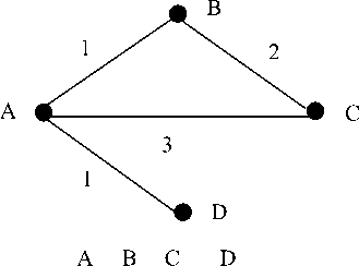
The connections in many networks are not merely binary entities, either present or not, but have associated weights that record their strengths relative to one another. In weighted networks the ties among nodes have weights assigned to them. Ties often have a strength naturally associated with them that differentiate them from each other. Tie strength has been operationalized as weights. A weighted network can be represented mathematically by an adjacency matrix with entries that are not simply zero or one, but are equal instead to the weights on the edges. Fig.1 shows an example of a weighted network and its mathematical representation. A few centrality measures have been proposed for weighted networks such as [8] [9][10]. However, those generalizations have solely focused on tie weights, and not on the number of ties. Zhao et al. [11] proposed a basic measure in weighted networks, h-Degree, it combines both tie weights and number of ties, which can be used to measure the centrality of the node. Furthermore, Zhao and Ye [12] promoted the concept of h-degree to the directional weighted network and introduced the directed h-degree. Zhai [13] proposed a communication centrality to measure node centrality reflecting a communication ability of a node which is suitable for the analysis of weighted undirected networks.

Most analysis and models have assumed that networks are static, typically represented in graph form as a number of nodes connected by edges. However in real life many networks are dynamic. New nodes are added to the graph, some existing ones are removed, and edges come and go too. Yet there are important networks whose topology changes rapidly, and its dynamic aspects have a significant effect on connectivity:

• -    Citation Networks: The vertices of a citation network are scientific papers and the directed edges of the network connect a paper to another if the former cites the later. The evolution of a citation network is therefore simple: A new vertex is added to the network for a newly published paper and links between this new paper and the papers it cites are added.

• -    Communication Networks: Several networks fall under the category of communication networks i.e. world wide web (WWW), the Internet. The nodes of the WWW graph are the homepages and the

  directed edges of the graph are the hyperlinks from one page to another.

  - Dynamic Networks in Computer Science: Several computer science application areas for dynamic networks. In logic programming languages, functional languages and data flow languages the given program is converted to a graph. This graph is changed over the time with the operations specified by the program hence representing a dynamic graph.

  While several static metrics have been defined and are widely used for SNA, dynamic metrics are a relatively new research field. In recent years several extensions of existing static centrality metrics to the dynamic case have been proposed such as [2][3]. D. Braha and Y. BarYam [4] studied how degree centrality evolves in a dynamic network by representing the network by time series. Thus far, the models and analytic tools used to characterize dynamic network behavior have been somewhat limited. It’s simple and common to look at static snapshots of the network independently, and use the average characteristics of all snapshots; for example, a possible way of estimating a node’s topological importance over time is to use the average value on the node’s centrality over all static snapshots. Such dynamic analyses, however, are limited since they neglect temporal paths that can cross over multiple temporal snapshots. In terms of dynamic graph, paths between nodes frequently exist by sewing partial paths between temporal snapshots. More recently, Tang et al. [5] proposed temporal centrality metrics based on temporal paths in order to effectively measure the importance of a node in a dynamic network. In addition, Kim and Anderson [6] extended the Tang’s proposal by introducing a new model called time-ordered graph which can reduce a dynamic network to a static network with directed flows. The temporal definition for degree, betweeness and closeness centrality metrics according to that model are also provided [6]. Federico et al. [7] proposed a new centrality measure called change centrality, which measures how central a node is with respect to the network changes.

  In this paper, a temporal communication centrality measure is presented. This measure is based on time-ordered weighted graph, to reflect the communication ability of a node in a weighted dynamic network. In section III, a description of a dynamic network, the time-ordered weighted graph and the proposed measure are introduced.

  
  
  

  A

  
  
  
  
  
  
  
  
  
  
  
  
  
  

  B

  
  
  
  
  
  
  
  
  
  

  C

  
  
  
  
  
  

  D

  
  

  Fig.1: weighted network and its matrix

  
  

  II. Related Work

  Network centrality diagnostics are designed to measure which nodes are important [1]. Depending on the application, the importance of a node can have different meanings and hence several network centrality measures have been proposed, namely degree, closeness and betweenness centrality [1]. Degree centrality focuses on the level of communication activity and defined as the number of links incident upon a node (i.e., the number of ties that a node has). The degree can be interpreted in terms of the immediate risk of a node for catching whatever is flowing through the network (such as a virus, or some information). Degree centrality of a node x can be formalized as:

  
  

  deg( x )

  C_D =

  N - 1

  
  
  
  

  where deg(x) is number of its links and N is the total number of nodes in the network. Betweenness centrality measures the number of times a vertex occurs on a geodesic (shortest path). Nodes that are between other nodes may control interactions between these other nodes. Betweenness centrality of a node x can be formalized as:

  
  

  C B =

  
  

  ^NN g ij ( x ) i = 1, i ≠ x j = 1, j-,j≠x    gij

  
  
  
  

  where g ij is the number of shortest paths from node i to j and g ij ( x ) is the number of these paths which passes through the node x . Closeness centrality is based on the idea that nodes with a short distance to other nodes can spread information very productively through the

  
  

network. Closeness centrality of a node x can be formalized as:

C C =    ^{N - 1}                (3)

∑ d(x, y) y≠x where d(x, y) is the shortest-path distance between actors x and y.

For unweighted networks where edges are just present or absent and have no weight attached, many centrality measures have been presented. There has been a growing need to design centrality measures for weighted networks, because weighted networks where edges are attached weights would contain rich information. Degree centrality was extended to weighted networks by Barrat et al. [9] and defined as the sum of the weights attached to the edges connected to a vertex. Lately, Opsahl et al. [21] proposed a new generation of vertex centrality measures for weighted networks, which takes into consideration both the weight of edges and the number of edges associated with a vertex.

One of the important centrality measures which is suitable for this research is called h-degree. The h-degree is defined as,” The h-degree (dh) of node n is equal to (dh) if dh(n) is the largest natural number such that n has at least dh(n) links each with strength at least equal to dh(n)” [11]. Greater h-degree of neighbor nodes indicates more powerful communication ability and greater influence. In citation networks, the h-degree refers to the most cited nodes. In co-author networks, it singles out the most collaborative authors. H-degree combined between social network analysis and the notion of h-index. The h-index [20] is an index that attempts to measure      both      the productivity and impact of the published work of a scientist or scholar. The index is based on the set of the scientist's most cited papers and the number of citations that they have received in other publications. The h-index can be defined as,” a scholar with an index of h has published h papers each of which has been cited in other papers at least h times”. Since this research is improved for dynamic networks and the time-ordered weighted graph is used, then the directed h-degree should be used to measure the importance of the neighboring nodes. The directed h-degree is define based on the directions of links, which naturally leads to the In-h-degree (hI) and Out-h-degree (hO), and can be defined as follows:

• •    In- h -degree (h_I) of node n is equal to h_I(n) if h_I(n) is the largest natural number such that n has at least h I (n) In-links each with strength at least equal to h I (n).

• •    Out- h -degree (h O ) of node n is equal to h O (n) if

h O (n) is the largest natural number such that n has at least h O (n) Out-links each with strength at least equal to h O (n) [12].

Li Zhai et al. [13] proposed a new node centrality measurement in a weighted network, the communication centrality, which is inspired by Hirsch’s h-index. Communication centrality considers two factors (edge weight and h-degree of the neighbor nodes), calculates their product and applies the h-index to balance the products and node degree.

While many social networks are dynamic in that they evolve over time and tie strengths are important in dynamic processes taking place on these networks, this paper presented the communication centrality measure but for dynamic networks which is called: Temporal Communication Centrality. And to be more precise in the centrality calculations in dynamic way, the time-ordered graph model proposed by H. Kim and R. Anderson [6] is extended for a weighted networks. This model is called, time-ordered weighted graph.

• III.    Methodology

To address the limitations of existing approaches discussed above, we propose the communication centrality for dynamic networks and provide an example for its computation. Furthermore, we introduce two derived metrics. The description for the dynamic model, time-ordered weighted graph and temporal communication centrality are introduced in this section.

• A.    Dynamic Model

A dynamic network is a network whose topology changes over time through addition or removal of edges and nodes. We assume that the time during a network is finite (from the start time t_min = 0 until the end time t max = T ).

A dynamic weighted network G^D 0,T = (V,E 0,T ,W) on a time interval [0, T ] consists of a set of vertices V , a set of edge weights W and a set of temporal edges E 0,T where a temporal edge (u, v) i,j ∈ E 0,T and its corresponding weight w uv exists between vertices u and v on a time interval [ i, j ] such that i ≤ t_max and j ≥ t_min .

A popular approach to represent dynamic networks is to construct a sequence of time windows, where for each window we consider a “ snapshot ” of the network at that time interval (We use ∆t to denote the size of each snapshot (or window size), for simplicity we assume that ∆t =1).

In other words, a dynamic network can be represented as a series of graphs G t , G t , . . ., G t . Then G t represents the aggregated graph which consists of a set of vertices V , a set of edge weights W and a set of edges E_t where this edge with its weight w_uv exists in G_t only if a temporal edge (u, v) i,j ∈ E 0,T exists between vertices u and v on a time interval [ i, j ].

For clarity, we introduce the following example. When t_m i _n = 0, t_max= 3 and At = 1, the dynamic network with the set of temporal edges and its weights as shown in Table 1 can be represented as the aggregated graph where all edges are aggregated into a single graph, G_t as in Fig. 2(a), and the series of static networks, G 1 , G 2 and G 3 as in Fig.2(b).

Aggregating over all edges as shown in Fig. 2(a) loses important temporal information that can help elucidate the structure of a dynamic network such as: frequency of events and the time difference between subsequent events. In time series representation it is difficult to directly analyze the temporal characteristics of a dynamic network from snapshots of the network as shown in Fig. 2(b). For example, if we may want to find a path from node A to F. We have to use one of the following paths:

A^B^C^E^F or A^B^D^E^F in the aggregated graph. In the series of networks we have to use the path from A to B then from B to D at t=1, then use the path from D to E and from E to F at t=2. But when dealing with the time-ordered weighted graph model, we can find no path from A to F in this interval as shown in Fig. 3. So we can say that time series representation cannot depict all temporal information.

Table 1. Example of dynamic weighted network edges

Temporal Edge	Time Interval	Edge weight
(A,B)	[1,1]	5
(B,D)	[1,2]	2
(B,C)	[2,2]	4
(D,E) , (E,F)	[2,3]	3,1 respectively
(C,E)	[3,3]	1

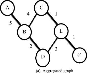
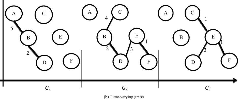
Fig.2. (a) static weighted graph (b) dynamic weighted graph

• B.    Time-Ordered Weighted Graph

The time-ordered weighted graph is constructed as shown in Fig.3 to capture all the connectivity information in the network, which has much richer information about the events described in Table 1.

Let Time-ordered weighted graph G = (V, E, W) is a directed weighted graph. It has a vertex vt for each v∈V where t E {0, 1,......, n}; it has edges from ut-1 to vtand from vt-1 to ut with the weights wu v ,wv u associated to those edges, respectively. It has edges from vt-1 to vt for all v E V and t E {1,...... , n}. In this paper, we consider the weighted networks whose edge weights are of natural number. We will also assume throughout this paper that all weights are non-negative. Negative weights are possible in some cases. They are, for instance, used sometimes in sociological studies of acquaintance networks to represent animosity between individuals.

The graph G = (V, E, W) is used to offer a definition for communication centrality to reflect the communication ability of the node in a dynamic weighted graph as follows.

• C.    Temporal Communication Centrality

Efficient communication means high impact (wide access or high reach) and low cost. Communication centrality considered three major influencing factors [13].

• 1.    Node degree: namely the number of neighbor nodes. Clearly, more neighbor nodes indicate more effective communication of a node since it can pass on and receive information through more channels.

• 2.    The communication ability of the neighbor nodes of a node: demonstrates the influence of its communication.

• 3.    Edge weight: has influence on the communication ability of this node.

The first and third factors are clear and easy to be determined from the network, but how can we reflect the communication ability of the neighbor nodes? In [13] the h-Degree is used to reflect this factor in the calculation of the communication centrality. However, in this paper we are dealing with a time-ordered weighted graph, which is a graph with directed flows, so we must use the directed h- Degree [12] to measure the communication centrality. In a directed weighted network, the In- h -degree ( h I ) of node n is equal to h I (n) if h I (n) is the largest natural number such that n has at least h I (n) Inlinks each with strength at least equal to h I (n) , and the Out- h -degree (h O ) of node n is equal to h O (n) if h O (n) is the largest natural number such that n has at least h O (n) Out-links each with strength at least equal to h O (n) .Table 2 shows the In- h -degree and Out- h -degree of the nodes of Fig. 3.

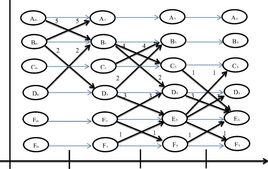
t=0                     t=1                      t=2                    t=3

Fig. 3. The corresponding time-ordered weighted graph of Table 1 on time interval [0, 3]

Table 2. The corresponding In-h-degree and Out-h-degree of the nodes of Fig. 2.

Tmie no de	t=0		t=1		t=2		t=3
	h I (n )	h O (n )	h I (n )	h O (n )	h I (n )	h O (n )	h I (n )	h O (n )
A	0	1	1	0	0	0	0	0
B	0	2	2	2	2	0	0	0
C	0	0	0	1	1	1	1	0
D	0	1	1	2	2	1	1	0
E	0	0	0	1	1	1	1	0
F	0	0	0	1	1	1	1	0

In this paper, an efficient approach to measure the communication ability of a node in a dynamic weighted graph. This approach based on the previous three factors with directed h-degree.

For each node there are channels between it and its neighbors. To measure the communication ability of the channel in the dynamic network, we will calculate the product of edge weight and directed h -degree, since we are using the time-ordered weighted graph, of each linked neighbor node in each time step. Then, we measure the communication centrality of a node in each time step according to the following definition.

Definition 1: Temporal Communication Centrality

Temporal Communication Centrality TCC(x) of a node x is the summation of communication centrality for all t∈{0,… … , n}, where the communication centrality c(x) of a node x at each time step is the largest integer k such that the node x has at least k In and Out-links satisfying the product of each neighbor node’s Out-h-degree at t-1 and the weight of the edge linked with node x and also the product of each neighbor node’s In-h-degree at t+1 (for all t∈ {1,… … , n}) and the weight of the edge linked with node x is no fewer than k.

TCC(x)=            : c(x)= max {k : wyho(y) at t-1 and wyhi(y) at t+1 k }                                   (4)

As an example we calculate the communication centrality of node D using the time-ordered weighted graph. At t=0, D0 is linked just with B1 and its weight with D0 is 2. The In-h-degree and Out-h-degree of B1 is 2, because it has 2 In-links and their weights are 5 and 2 and it has also 2 out-links and their weights are 4 and 2. Then we calculate the products of directed h-degree of B1 and its edge weight with D0. It can be seen that D0 has at least 1 neighbor node whose product is no less than 1. So the communication centrality of D0 is 1. Also for D1 which has In-link with B0 and its weight with D1 is 2 ( where ho(B0)=0) ,and it has 2 Out-links with B2 and E2 and their weights with D1 are 2 and 3 respectively (where hi(B2)=2  hi(E2)=1).  So the communication centrality of D1 is 3. Similarly, the communication centrality of D2 and D3 are 3 and 1 respectively. So the temporal communication centrality of D is 1+3+3+1=8. Table 3 shows the communication centrality of each node in each time step and the temporal communication centrality.

We notice that In-h-degree of each node at t=0 is always will be 0 because there is no in-links, and also for Out-h-degree at t=n because there is no out-link.

Table 3. The communication centrality of each node in each time step and the TCC(x)

Time nodes	c(x)				22 ^^
	t=0	t=1	t=2	t=3
A	1	1	0	0	2
B	2	2	2	0	6
C	0	1	1	1	3
D	1	3	3	1	8
E	0	1	1	1	3
F	0	1	1	1	3

To compare the node centralities in different networks, the centrality indexes of nodes in different networks should go through standardized definition to gain the standardized centrality measurement. The temporal communication centrality can be standardized by dividing each node communication centrality by (|N|-1).m where m = j - i .

S£_oc(x)

So, TCC(x) = (5)

So the temporal communication centrality of nodes A-F are 0.13, 0.4, 0.2, 0.53, 0.2, 0.2.

• D.    Derivative Measure of Temporal Communication Centrality

In this section, we will define two derivative measure related to the TCC measure proposed in the previous section. They are iterative communication centrality c⁽ⁱ⁾(x) and Temporal communication centrality TCC^{(i )} ( where i ≥ 2).

In order to more accurately measure the importance of the neighbor nodes in calculating the TCC , we can apply the method of TCC in the neighboring nodes and calculate their communication centrality and replace the neighboring node directed h-degree with its communication centrality at each time step, which can be called c (x) of second order (c⁽²⁾( x )) and their summation are called TCC(x) of second order ( TCC ⁽²⁾). Similarly, in order to obtain TCC of third order we take c( x ) of second order as the measure of the importance of the neighbor node. We can also define TCC of fourth order, etc.

Definition 2: Iterative Temporal communication Centrality

The iterative temporal communication centrality , noted as TCC⁽ⁱ⁾ , of a node x is the summation of iterative communication centrality c ⁽ⁱ⁾(x) (where i ≥ 2) for all t ∈ {0,… … , n}, where the iterative communication centrality of a node at each time step is the largest integer k such that the node x has at least k neighbor nodes satisfying the product of each node’s c ^(i-1)(x) and the weight of the edge linked with node x is no fewer than k .

As an example, we will calculate both c ⁽²⁾(x) and TCC⁽²⁾ of node B. At t=0, B has two neighbors, namely A 1 and D 1 whose communication centrality are 1 and 3 respectively. Then we calculate the product of their communication centrality and the weights associated to them with B 0 . We can see that B 0 has at least 2 neighbors whose products are no less than 2.So c ⁽²⁾(B 0 ) =2. Also for B 1 which has four neighbors, namely A 0 , D 0 , C 2 , D 2 whose the product of their communication centrality and their weights with B₁ are 5, 2, 4, 6 respectively. So we can see that B₁ has at least 3 links whose production is no fewer than 3. So c ⁽²⁾(B 1 ) =3. Similarly, c ⁽²⁾ of B 2 and B 3 are 2 and 0 respectively. So the TCC⁽²⁾(B) is 2+3+2+0= 7. Table 4 shows both c ⁽²⁾ and TCC⁽²⁾ of the nodes of Fig.2.

Table 4. The iterative measures of second order

Time nodes	c (2)(x)				TCC(2)
	t=0	t=1	t=2	t=3
A	1	1	0	0	2
B	2	3	2	0	7
C	0	1	1	1	3
D	1	3	3	1	8
E	0	1	2	1	4
F	0	1	1	1	3

• IV.    Conclusion

Based on the well-known measurement directed- h-degree and the notion of time-ordered graph , this paper proposes a new approach to calculate the Temporal Communication Centrality. The proposed approach is designed to overcome the limitation of Li Zhai, which introduced a centrality metric for static networks, in which to reflect the communication ability of a node in dynamic networks since many social networks are dynamic in that their topology changes rapidly. Also derivative measures are represented depending on the proposed measure.