Company management system estimation on the basis of adaptive correlation to the environment

After the global crisis outbreak companies have changed a lot: stronger integration of companies, lead to numerous consolidations, acquisitions and mergers.

The Russian companies are not an exception. Holdings (hereinafter referred as to production systems) will be a general moving force, which diversified scope of the activity and the work was in hand inside. It is a gathering moment, but the other process has not completed yet – creating the model of decision-making system. If it is, Russian companies can be considered well-functioning systems and not just a collection of heterodeneous assets [1].

A holding company manager will find the following difficulties, when managing the holding companies the decisionmaking system of holding (further production system):

• –    intercommunication between the companies is inaccurate measurement, subjectivity;

• –    intercommunication between accounting system and decision-making system;

• –    a lot of complex methods of decision-making system;

• –    holding companies have different development vectors and conflicting purposes.

One original way is correlative adaptation which was described for physiology of group’s humans in hard living conditions (far North city, polar expedition, or a hospital, for example) in 1985 by A. N. Gorban, E. V. Smirnova.

The crucial question is: what is the resource of adaptation? This question arose for the first time when Selye published the concept of adaptation energy and experimental evidence supporting this idea [1; 2].

In modern “Encyclopedia of Stress” it is written: “As for adaptation energy, Selye was never able to measure it...” [3].

After that their work (A. N. Gorban, E. V. Smirnova, T. A. Tyukina ) was published in May 2009, they have been studing ensembles of similar systems under load of environmental factors. The phenomenon of adaptation has similar properties for systems of different nature. Typically, when the load increases above some threshold, the adapting systems become more different (variance increases), but the correlation increases too. If the stress continues to increase the second threshold appears: the correlation achieves maximal value, and starts to decrease, but the variance continues to increase. In many cases this second threshold is a signal of fatal outcome approaching.

This effect is proved by many experiments and observations of groups of humans, mice, trees, grassy plants, and on financial time series. A general approach to explanation of the effect through the dynamics of adaptation is developed. H. Selye introduced the term “adaptation energy” for explanation of adaptation phenomena. They formalized this approach in factors – resource models and developed models hierarchy of adaptation. Different organization of interaction among factors (Liebig’s versus synergistic systems) leads to different adaptation dynamics. This gives an explanation to qualitatively different dynamics of correlation under different types of load and to some deviation from the typical reaction to stress.

In addition to the “quasistatic” optimization factor – resource models, dynamical models of adaptation were developed, and a simple model (three variables) for adaptation to one factor load was formulated explicitly.

In economics, we use the published results of data analysis for equity markets of seven major countries over the period 1960–1990 and for the twelve largest European equity markets after the 1987 international equity market crash. Some of the results obtained in econophysics [4] also support our hypothesis.

We study micro economic systems (hereinafter referred as to production systems-companies). In our research work we have considered data of economic systems (special case is development sector) since 2004. In April 2008 we applied the program of decision-taking system estimation in economic system (SM. city) [2].

For it we completed the following problems:

• –    made mathematical formulation the discrete- multivariate system for economic system (hereinafter referred as to production systems-companies);

• –    made calculations and analyzed plan/fact of sample estimation correlation matrixes, correlation graph G ;

• – made resources allocation (special case is cash) among functions of economic system.

Making mathematical formulation the discrete-multivariate system for economic system (hereinafter regarded for as production systems-companies). Follow the systems theory (R. Kalman and other, 1971) representable system S consider

S = { T , X , V , h , ф ) .                   (1)

The notation:

T = {t / t = 0,1, 2,...} - discrete set of time (window of time).

X –    phase     space of     system,

x ( t ) = [ x 1 ( t ), x ²( t ),..., x n ( t )] ^T e X - n - variable phase vector,            state            vector,            and

x * ( t ) = [ x *’ ( t ), x * ²( t ),..., x * ⁿ ( t )] ^T e X - n - variable phase vector, suboptimal estimation by R. Bellman.

The variable phase vector of economic system is xⁱ ( t ) – financial expenditure for the functions (describe all action, business process) of economic system. There are unification accounts, functions in special program. Study table 1 as an example. For the research 417 functions (the variable phase vector of economic system) were used.

V – space analytic estimates of system, V ( t ) = [ v 1 ( t ), v ²( t ),..., v^s ( t )] ^T e V - 5 - vector analytic estimates.

ф : T x X ^ X - transition functions of system, is:

x ( t + 1) = ф ( x o , x ( t )),                 (2)

where x ₀ = x (0).

h : T x X ^ V - function analyzes the space of points (observation function), is:

v ( t ) = ^( x ( t - 1), x ( t - 2),..., x ( t - k )).        (3)

Use the variable phase vector x ( t ) for prior periods. The parameter k is depth horizon (in our special case k = 6 months). Matrix is defined

The accounts, functions

Table 1

Name of project Activity category Item of income/expenses Subclause of income/expenses Functions of S (variable phase vector) ( xi ) Plan x*n(t) Fact xi(t) Project 1 Investments Capital outlays Development planning Development planning The water-system design x1 x*1(t) x1(t) Day-to-day operation, Finances Disposition    of profits Profit-and-loss last years Inventory x2 x*2(t) x2(t) Day-to-day operation, Principal activity Operating activities Services of other company Other services of other company Other x3 x*3(t) x3(t) xn (t -1)

x n ( t - 2)

The sample correlation matrix R_k ( t ) for observation function is:

. (4)

v ( x ( t - 1), x ( t - 2),..., x ( t - k )) = R k ( t ).           (9)

X T ( t - 1)

X T ( t - 2)

...

X T ( t - k )

x 1 ( t - 1) x ²( t - 1) x '( t - 2) x ²( t - 2)

...                          ...

x ’( t - k )   x ²( t - k )

x n ( t - k )

Execute centering and normalization components of matrix Xk ( t ). Then
	o x	( t - 1)		o x '( t - 1)	o x 2( t - 1) .	o .    x n ( t - 1)
o X k ( t ) =	o xT	( t - 2) ...	=	o x 1 ( t - 2) ...	o x 2( t - 2) . ...                     ..	o .   x n ( t - 2) .            ...	(5)
	o [ xT	( t - k ) J		o x 1 ( t - k )	o x 2( t - k ) .	o . x n ( t - k ) _

^o         o         o

X T (t ) = x ( t - 1) x ( t - 2)

o

x ( t - k )

x 1 ( t - 1) At - 2) ... x 1 ( t - k ) x 2 ( t - 1) At - 2) ... At - k )

The observation function is integral representation action of the system. We have opportunity to the analyze the behavior of multivariate system, so we find and control change evolved from the company operation as well as caused by management and exopathic.

Then we single out correlation indicators. Indicators is graphs G_i ^sum_total ( t ) – absolutely summable of sample correlation coefficients i ’s function this other, G_i ^sum_neg ( t ) – sum negative of sample correlation coefficients and G_i ^sum_plus ( t ) – sum of sample correlation coefficients is more than 0, G_i ^difference ( t ) – sum of sample correlation coefficients. Change for window time the G shown figure 1.

n

_G sum_total( t ) = T| r j (t )|:(| r j ( t )|> r _sign),        (10)

j = 1

o          o               o

_x n ( t - 1) x n ( t - 2) ... x ( t - k )_

n

_G s_um_pi_US( t ) = T r j (t ): ( , ..( t )| >  r sign ) n ( r j (t ) >  0),   (11)

j■ = 1

o        o and calculate Rk (t) = —у Xk (t)XT (t) = Jr (t)||

n

_Gi Surn_„e_g ( t ) = T r ( t ) : ( r ( t )| >  r sign ) ^ ( Г у ( t ) <  0), (12) = 1

i , j = 1, ..., n ,                                  (7)

G difference ( t )    g sum_plus ( t ) । g sum_neg ( t )

where j t ) = — УД t - l ) x°^j ( t - 1 ). (8) k ^{- 1} 1 = 1

Value r_ij ( t ) is a sample correlation coefficient (Pearson coefficient) between variables xⁱ ( t ) and x^j ( t ) of window time t and R_k ( t ) – sample correlation matrix between the variable phase variable of window time t for depth horizon k .

Thereby (4, 5) diagonal matrix R_k is г ( t ) = 1 for all i , j' = 1,..., n . and all t , and other coefficient from -1 to +1 (^{-1 5} r j ⁵ 1).

On the basis of sample correlation matrixes (7) we create correlation graph of the system G_i ( t ). Show relationship among the functions of the system figure 2 and figure 3.

where r _sign – significance of sample correlation coefficient for data of sample correlation matrix with parameter k which is depth horizon.

All graphs G_i ( t ) account for window time T including the relationship between functions of the system figure 2, figure 3.

Made calculations and analyzed plan/fact of sample correlation matrixes, correlation graph G . Figure 1 shows the important events in economic system.

• 1.    Drawing up/making up an estimate – the budget of construction.

• 2.    Getting a permit for construction – the document authorizing the start of project construction and favorable for obtaining a bank loan.

• 3.    Creating the TQM – creating regulations and standards for the company.

• 4.    Getting finance – getting a loan from the Savings bank («Sberbank»)

• 5.    Starting the project construction – starting the construction of residential property.

• 6.    Creating similar/identical/analogous hereinafter production system-companies .

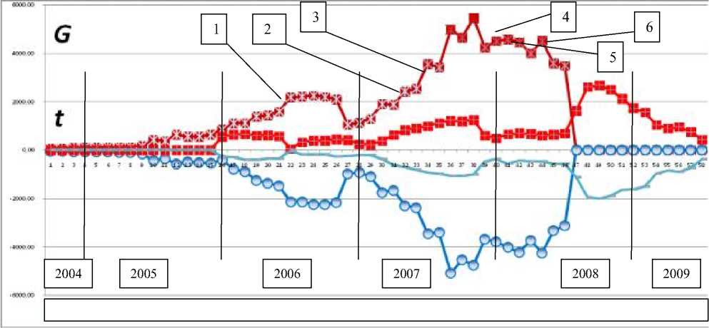
Fig. 1. The diagram variable phase vector of economic system in dynamics

The larger the value of G_i ^sum_total( t ) is, the larger crisis our system experiences.

The functions involved in the economic activity of the production system are interrelated (figure 2).

Within the reported/determined period you can analyze separate functions and determine their influence on the system (figure 3). After that you can find principal functions for allocating money in the company (table 2) [5].

Resources allocation (special case is cash) between functions of the economic system. Functions that have high correlation get more money. The method of R. Bellman is used for financial allocation among corporate objectives, strategies and functional systems (table 2).

The article described the method to get control of heterogeneous assets.

You can use it – to determine and fix the period of stress in economic system (hereinafter reffered to as production systems-companies); to optimize the process of management; to allocate resources (special case is cash) between functions of economic system.