Comparative analy-sis of verified numerical simulation of cavitation based on the Rayleigh – Plesset model for liquid propellant rocket engine pumps

The operation of a turbopump unit (TPU) as part of a liquid-propellant rocket engine (LRE) is characterized by increased requirements for ensuring operability and maintaining main parameters at a given resource. The main purpose of a TPU is to ensure a continuous supply of fuel components to an engine combustion chamber. A number of factors can affect the operation of a TPU, for example, local decrease in fluid pressure that occurs when the pump blade profile flows around. This part of a pump may be the site of cavitation. Cavitation is a phase transition of a liquid into a gas inside a liquid at a certain temperature and pressure, which occurs in a moving liquid due to local pressure drops to saturated vapour pressure. The instability of the TPU operation in the cavitation mode due to the violation of the medium continuity mode can affect the efficiency and the generated specific impulse of a rocket engine [1].

When designing a TPU, it becomes necessary to conduct a series of model tests in order to refine pump parameters, as well as to confirm the anti-cavitation qualities of the pumps. The testing of pump operation modes under the influence of cavitation can be performed both on test facilities with testing on a model liquid, and using various numerical simulation methods in computational fluid dynamics (CFD) programs. Currently, there are a fairly large number of different software packages that allow us to simulate cavitation numerically in the flow around the blades of pumps, turbines, a hydrofoil of a watercraft, or during fluid flow in various complex geometries. The simulation of cavitation flow can be a good addition to field tests. Nevertheless, despite the large database of tests that have already been carried out, the increased energy density of a TPU as an LRE unit raises the question of approximating the current data to the simulation of the flow in the pump.

The ANSYS package for modeling a cavitation flow presents a number of models based on the Rayleigh-Plesset equation. This paper considers the results based on the application of the Zwart-Gerber-Belamri cavitation model, which is compatible with all turbulence models available in the ANSYS package. Like all models of a physical phenomenon, it has a number of limitations[2]:

• –    it is assumed that there is a mass transfer between the liquid and vapour phases. The cavitation model takes into account both bubble formation (evaporation) and collapse (condensation);

• –    the cavitation model takes into account the growth of a single vapour bubble in the liquid;

• –    the default model does not take into account the influence of non-condensable gases.

Theoretical model

Before analyzing the data, let us consider the equations included in the Zwart-Gerber-Belamri model based on the Rayleigh-Plesset equation. For the first time, this equation, which describes the complete transformation of work (performed by the mass during the collapse of the cavity) into kinetic energy, was presented in [3]:

^p l RR TT

+ ³ R 2

2 ^T

- P ,

where p – pressure; R – bubble radius; ρ – the density of the liquid around the vapour bubble; R_T and R_TT – derivatives of the radius with respect to time. In [4], Plesset presented an equation describing the growth of a gas bubble in the liquid and being derived from the moment equations:

„ d 2 ^r b ,3 ( ^dR B      2 o    P v - P

RB —;—+_ lI +--=-----, dt2   2 ^ dt J   pf RB    pf where R – bubble radius; p – pressure in the bubble (it is assumed that it is vapour pressure at fluid temperature); p - pressure in the liquid surrounding the bubble; pу - liquid density; о - surface tension coefficient between liquid and vapour.

In the ANSYS software package, this model is simplified [2]. It does not take into account the surface tension force and all second-order equations, since these equations are used for low-frequency vibrations d ^ B dt

2 P v — p V ³ p у

It is this model that was considered by the authors Philip J. Zwart, Andrew G. Gerber, Thabet Belamri in the article [5]. Expressing the number of bubbles in terms of N B , the volume fraction of vapour per unit volume can be expressed as

4 з rv = VbNb = J nRB Nb ,

where R_B – radius of a bubble in the fluid. The total rate of interfacial mass transfer due to cavitation per unit volume will be equal to

S lv =

3r_v P v 2 P - P R b v p i

For the case of condensation, the equation is expressed as follows:

S lv

= f 3 r v P v

R B

2 I P - P

- ^—s_sgn( ( P, - P ), 3    P i

where F – empirical calibration factor. Assuming that cavitation bubbles do not interact with each other, the authors of [5] replaced r v with r nuc (1 – r v ) for the case of evaporation, where r nuc is the volume fraction of the cavitation bubble formation center. The final view of the cavitation model is the following:

S lv = ]

P  ³ r nuc ^{(1 -} r v ) P v \ ^{2 P} v ^{- P} p^p

F vap -----о------Jz------ if ^P <  ^P v ,

RB      V³ P/

F , cond

3 Г P v  - P - P v

R b V P i

i f P >  P v .

The following values are applied for this model: R b = 10^–6 m, r nuc = 5 · 10^–4, F vap = 50 and F cond = 0.01.

The above cavitation model is included in the vapour transport equation:

d

— ^(a P v ) + V ⁽ a P v V v ) = R„ ^- R_c ,                              ⁽⁸⁾

dt where α – vapour volume ratio; ρν – vapour density; Vν – vapour phase velocity; Re, Rc – sources of mass transfer associated with the growth and collapse of vapour bubbles, respectively (modeled based on the Rayleigh-Plesset equation).

We also consider the equations included in a turbulence model. It is known that the flow of liquids and gases in nature can be divided into two types: laminar and turbulent. The first flow is characterized by the stability of parameters or, in extreme cases, the smoothness of their change. For a turbulent flow P. Brandshaw gives the following definition of turbulence [6]: 'Turbulence is a three-dimensional non-stationary motion in which, due to the stretching of vortices, a continuous distribution of velocity pulsations is created in the range of wavelengths from the minimum determined by viscous forces, to the maximum determined by the boundary conditions of the flow.'

The turbulent flow models used in ANSYS are based on the theory of L. Prandtl and the work of A. N. Kolmogorov. Prandtl's theory is based on the calculation of the displacement of the flow through the ratio of the rate of momentum transfer between adjacent layers to the length of the elementary area, and the transfer rate is the transverse pulsation velocity. Kolmogorov in [7] proposed a system of equations for the turbulent regime, which formed the basis of the model described below. In the article [8], the authors B. E. Launder and D. B. Spalding described the turbulence model based on the system from the equation for the kinetic energy of turbulence k :

^{d (} P ^k ) d t

d           d  |     u

+ ^⁽P u i k) = ^ M + — ^d x i          ^d x j l   о k

d k d x j

⁺ G k ⁺ G b

^{- p e-} Y M ^{+ S} k •

The equation for the value of e (turbulence energy dissipation rate) can be obtained from the Na-vier-Stokes equation, but this equation is not closed. For closure, it is necessary to present the equation in the following notation:

5 ( p£ ) ₊ d ( p£ u i ) ₌ 5 d t       d x i      d X j ^

ц ц + —

^

de

5 X;

e ²

⁺ C E 1 ( G k ⁺ C 3 e G b ) - C _£ 2 ^p7 ⁺ S E . k

In these equations, μ t = ρ C μ k ²/ε – coefficient of virtual viscosity; G k – turbulence kinetic energy gain due to mean velocity gradients; G b – turbulence kinetic energy gain due to bouyancy; Y M – the contribution of fluctuating dilatation in compressible turbulence to the total dissipation rate. C ε1 , C ε2 and C ε3 are constants; σ k and σ ε – turbulent Prandtl numbers for k and ε respectively; S k and S ε – assignment values. In ANSYS [2] for the constants the following values are accepted: C ε1 = 1,44, C ε2 = 1,92 and C μ = 0,009, σ k = 1,0 and σ ε = 1,3.

It is important to note that the article [5] draws attention to the fact that standard turbulence models cannot correctly predict the oscillatory behavior of the flow. For this, the authors used the modified formula for the turbulent viscosity coefficient

Ц tm = f ( P ) C ц —,                                  (11)

e where f(P) = Pv + ((Pv - Pm )/ (Pv - Pl))n • (Pl - Pv ).

Consideration of statistics on tests of various pumps

It should be noted that in the geometric models being considered, a prepump was not used to improve the anti-cavitation qualities of the pump (in the paper [9] it was used in the experiment, but not in the model). In model tests of the TNA of an LRE, the pre-pump was installed, which also needs to be reflected in the geometric model in the numerical simulation of the cavitation flow.

In the paper [5] (which presents the Zwart-Gerber-Belamri model for the first time) the authors also consider the application of this model to a geometry similar to the pumps being considered (the case of cavitation in the prepump). The experimental data are compared with the simulation. The authors note that near the nominal operating mode (Q / Qn = 1.03), the head fall on the curve occurs faster and simultaneously with experimental measurements.

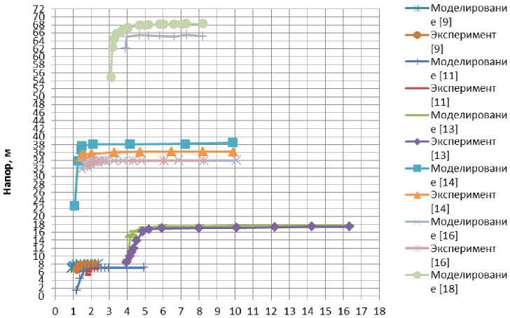
In the paper [9], the authors consider the issue of numerical simulation of oscillations in a centrifugal pump at low flow rates. The RNG k-ε model is used as a turbulence model. The design parameters are also presented in the table. The results of hydraulic tests are shown in Fig. 1. The authors carry out calculations in the ANSYS CFX environment with the number of cells 1562765. They also compare the obtained heads H with the number of cells 1562765, 1837613, 2129429, 2375885, 2629005. The head with the number of cells 1562765 will differ from the head with the number of cells 2629005 by 1.008535 times, which indicates a small effect of the number of cells on the accuracy of the calculation, if their sum exceeds a certain limit.

NPSH (Net Positive Suction Head) value in Fig. 1 is net hydraulic head or positive suction head measured by the height of the liquid column at the inlet to the pump, NPSHa is an available head value at the pump inlet pipe minus the pressure of the saturated vapour of the liquid

NPSHa = pn- + u n - pi- ,                         (12)

Pig  2 g  Pig where pin – pump inlet pressure; иin – pump inlet speed; pν – saturated vapour pressure.

In the paper [10], as a basis for comparison, the authors take the data of the hydraulic flow of the designed centrifugal pump, the design parameters for which are presented in the table. The turbulence model RNG k-ε, modified on the basis of Johansen's idea, is chosen as a turbulence model. The obtained parameters for the nominal mode are presented in Fig. 2. The analysis of the parameters shows good agreement between the experimental data and the simulation results. The authors consider that the reasons for the discrepancy are the following:

– lack of consideration of the gap clearance between the blades and the body, losses due to water expansion in the outlet collector;

–assumptions made in the available cavitation model.

NPSHa, м

Рис. 1. Сводный график напоров

• Fig. 1.    Summary head graph

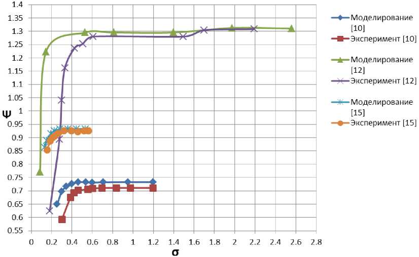
Рис. 2. Сводный график чисел кавитации

• Fig. 2.    Summary graph of cavitation numbers

The value Ψ – head coefficient; it is expressed by the following formula

H

Ψ= ₂, u ₂ 2 g

where H – pump head; u2 – circumferential speed at the outlet. The number of cavitations σ is expressed by the formula pin - pv σ= in    v .

The article [11] studies pressure fluctuations in a pump under cavitation mode. The RNG k-ε model is used as a turbulence model. The paper presents a geometric model of the pump, similar to the model from the article [9], but the operating mode was considered at a nominal flow rate. The data on the results of a real experiment and numerical simulation are shown in Fig.1. The grid being used for calculations consists of 1.56 million elements.

The paper [12] also studies cavitation phenomena in a centrifugal pump. The SST k-ε model is used as a turbulence model. In the study, the authors chose a model of a centrifugal pump with a small value of the coefficient of speed, the design parameters of which are given in the table. The results of hydraulic tests are shown in Fig. 2 (the value of Ψ was calculated from the available data in the article, since only the head value is given in the article). The grid being used for calculations consists of 1180228 elements.

The paper [13] studies the effect of cavitation on pump performance. The authors chose to study the AP1400 pump, which has a high flow rate. The turbulence model being used is RNG k-ε. The data on the results of a real experiment and numerical simulation are also shown in Fig.1. The computational grid consists of 5.9 million elements.

The paper [14] studies the performance and cavitation flow in the pump. The authors used a geometric model of the pump, the design characteristics of which are presented in the table. The SST k-ε model is used as a turbulence model. The graph of numerical simulation and experiment is shown in Fig. 1 (in [14] along the y-axis, the ratio of heads is indicated; for the graph, the value of the head from the article, multiplied by Hd, is taken). The computational grid consists of 3.02 million elements.

The paper [15] studies the effect of cavitation on an improved pump wheel blade. The authors used a geometric model of the pump, the design characteristics of which are presented in the table. The graph of numerical simulation and experiment is shown in Fig. 2. The authors also compared the resulting head with different numbers of elements in the geometric model: 5, 9.1, 12 and 20 million. The results show a maximum head coefficient deviation of 1.12%. The grid being used consists of 12 million elements.

The paper [16] stuies the issue of modeling cavitation in a pump. The SST k-ε model is used as a turbulence model. The graph of numerical simulation and experiment is shown in Fig. 1. Similarly to the previously considered work [14], in [16] the ratio of heads is indicated along the y axis. For the graph in Fig. 1, the pressure value from the article multiplied by Hd is taken. The design characteristics of the pump are presented in the table. Based on the works carried out by the authors in [17], it is claimed that the solution is relatively independent on the number of grid elements. In this regard, in the calculation model of the pump in the article [16], a grid of 5207832 elements is used. The authors also claim good convergence of practical results with simulation results.

The paper [18] considers cavitation in double inlet pumps. This design of the pump impeller is also used in the design of TPU for LRE rockets. The authors chose the ES8-300KPS double-sided inlet pump for the study. The k-ε model is used as a turbulence model. The graph of numerical simulation and experiment is shown in Fig. 1, the design characteristics of a double inlet pump are presented in the table. The computational grid consists of 4198349 elements.

Comparison Table of Pumps

№ п/п	Paper/pump	Characteristics	Value of a parameter
1	The designed pump from the article [10]	Nominal flow rate	32,8 m3/hr
		Pump speed coefficient	135
		Angular rate	1450 rpm
		Number of blades	5
		Outer diameter D 2	0,169 m
		Outlet wheel width	0,014 m
2	The designed pump from the articles [9] and [11]	Nominal flow rate	25 m3/hr
		Head	7 m
		Angular rate	1450 rpm
		Number of blades	7
		Inner diameter D 1	50 mm
		Outer diameter D 2	160 mm
3	The designed pump from the article [12]	Nominal flow rate	8,6 m3/hr
		Pump speed coefficient	32
		Angular rate	500 rpm
		Number of blades	6
		Outer diameter D 2	310 mm
		Inner diameter D 1	80 mm
4	Pump AP1400 [13]	Nominal flow rate	1385 m3/hr
		Head	17,8 m
		Angular rate	1485 rpm
		Number of blades	18
5	The designed pump from the article [14]	Nominal flow rate	25 m3/hr
		Head	36 m
		Pump speed coefficient	60
		Angular rate	2900 rpm
		Number of blades	5
		Outer diameter D 2	172 mm
		Inner diameter D 1	65 mm
		Outlet wheel width	12 mm
6	The designed pump from the article [15]	Nominal flow rate	200 m3/hr
		Head	20 m
		Angular rate	1450 rpm
		Number of blades	6
		Outer diameter D 2	270 mm
		Inner diameter D 1	150 mm
		Outlet wheel width	30 mm
7	The designed pump from the article [16]	Nominal flow rate	50 m3/hr
		Head	34 m
		Angular rate	2900 rpm
		Number of blades	6
		Pump speed coefficient	88,6
8	The designed pump ES8-300KPS from the article [18]	Nominal flow rate	820 m3/hr
		Head	64 m
		Angular rate	1480 rpm
		Number of blades	6

Let us consider the graphs in Fig. 1. If we take a 3% head drop as the start of cavitation, then we can draw the following conclusions:

• 1.    The beginning of cavitation for simulation is fixed at a lower value of NPSHa compared to the experiment, but at higher pressure for [9; 13; 14; 16; 18].

• 2.    The beginning of cavitation for modeling is fixed at a higher value of NPSHa compared to the experiment and at higher pressure for [11].

• 3.    At the cavitation start point, the difference in NPSHa relative to the experiment is less for the papers [9] by 10%, [13] by 6%, [14] by 6%, [16] by 15%, [18] by 10%.

• 4.    At the cavitation start point, the difference in NPSHa relative to the experiment is greater for the paper [11] by 6%.

• 5.    At the cavitation start point, the difference in heads relative to the experiment is greater for the papers [9] by 5 %, [11] by 3 %, [13] by 2 %, [14] by 6 %, [16] by 0,3 %, [18] by 4,5 %.

Let us also consider the graphs in Fig. 2. If we take a 3% drop in pressure as the beginning of cavitation, then we can draw the following conclusions:

• 1.    The beginning of cavitation for modeling is fixed at a smaller value of σ, but at a larger Ψ for [10; 12; 15].

• 2.    At the cavitation start point, the difference σ relative to the experiment is less for [10] by 18%, [12] by 62%, [15] by 8%;

• 3.    At the cavitation start point, the difference Ψ relative to the experiment is greater for [10] by 3%, [12] by 0.2%, [15] by 0.7%.

Conclusion

Based on the results of consideration of the mentioned papers, the above graphic materials and data on computational grids, we can make the following conclusions:

• 1.    Numerical simulation of the cavitation flow shows satisfactory convergence for the values of pump heads. These indicators remain stable even for large pressure values. The divergence of parameters when simulating cavitation in a double-inlet pump is similar to the divergence of the parameters for models with a single inlet.

• 2.    The data on the values of σ and NPSHa with respect to the head differ for the worse, since some works have shown a major discrepancy between the experimental data and the flow simulation data.

• 3.    The number of grid elements has a lesser effect on the accuracy of numerical simulation, since the difference between models with a larger and smaller number of cells is insignificant.

The conclusions mentioned above must be taken into account when applying the Zwart-Gerber-Belamri model for the numerical calculation of the hydraulic cavitation flow in the pumps of the TPU of an LRE.