Comparative Analysis of Explainable AI Frameworks (LIME and SHAP) in Loan Approval Systems

Published Online on December 8, 2025 by MECS Press

Technology is gradually taking over several walks of life, with Artificial Intelligence (AI) taking the lead in various domains. We find AI applicable in health, finance, education, business, and defense, among others. Today, people can utilize AI in ways believed to be impossible years ago. Loan approval systems are a strategic aspect of the financial industry, enabling individuals and businesses to access funding for various purposes. The use of machine learning algorithms in loan approval systems has become increasingly prevalent due to the growth of big data and the increasing complexity of financial transactions. However, one of the significant challenges with the use of these algorithms is their lack of transparency and interpretability, which can lead to biased or unfair loan approval decisions. To address this problem, explainable AI (XAI) frameworks have been developed to provide interpretable explanations for machine learning models [1]. The problem of interpretability and understanding how these systems work is called the “black box problem” in loan approval systems. The black box problem refers to the lack of transparency and interpretability in the prediction process of complex machine-learning models [2]. XAI frameworks enable users to understand how the model arrived at its decisions, making it possible to detect and address biases, errors, or inconsistencies in the decision-making process [3]. XAI frameworks for machine learning models such as Local Interpretable Model-Agnostic Explanations (LIME) and Shapley Additive Explanations (SHAP) have been used in XAI tasks with distinctive capabilities. LIME provides model-agnostic explanations by approximating a complex model with a simpler one that can be more easily explained. SHAP, on the other hand, assigns values to each feature's contribution to the model's output, providing a clear and interpretable way to understand the model's decision-making process. While these XAI frameworks have been applied in various domains, including healthcare, marketing, and finance, their effectiveness in loan approval systems remains under-explored. Thus, there is a need to evaluate the performance of these frameworks in loan approval systems and compare their effectiveness in providing transparent and interpretable explanations [4]. This study seeks to fill this gap by performing a comparative analysis of LIME and SHAP in loan approval systems to determine their strengths and limitations answering the following research questions: (1). How do LIME and SHAP perform in terms of explaining loan approval decisions made by a Random Forest model? (2). Which explainability framework (LIME or SHAP) provides better interpretability in loan approval systems? (3). How do LIME and SHAP compare in computational efficiency when applied to loan datasets? Overall, the study contributes to developing more trustworthy and transparent AI systems in the financial sector, promoting fairness and accountability in loan approval processes. The rest of the paper is organized into the following sections: Section 2 presents related work to the research. Section 3 covers the methodology of our study. The implementation experiments are carried out in Section 4, and Section 5 presents the conclusion and future research direction.

2.    Related Works

The use of automated processes or systems in critical decision-making has evolved. Critical systems and services such as health care diagnosis, infrastructural systems, high-risk financial services, and several others have adopted systems and solutions that do not only rely on human efforts [5]. In financial critical systems like loan credit scoring and predicting loan approvals and rejections, artificial intelligence models have been used for such tasks. What remains a challenge is how transparent the system’s results are to the concerned stakeholders [6]. This has given rise to Explainable AI which seeks to make the models more interpretable. Explainable AI is applicable in several fields today. In healthcare, it assists healthcare professionals in understanding and rationalizing the decisions made by AI systems when it comes to diagnosing ailments and suggesting treatment strategies [7]. Trust and safety in autonomous vehicles are strengthened by offering comprehensible explanations for the decisions made by the AI algorithms that govern these vehicles, thereby increasing acceptance and reducing uncertainty among passengers [8]. Explaining AI systems’s decisions in the legal profession enables judges and lawyers to understand the factors contributing to AI-generated outcomes. This ensures fairness, accountability, and transparency in legal proceedings [9]. Interpretation approaches are useful in unraveling the complexities of understanding AI systems, especially in the generation of synthetic data and other generative processes enhancing transparency [10]. By offering interpretable explanations, AI systems enable the identification of suspicious patterns, clarification of risk classifications, and the establishment of transparency in regulatory reporting. Financial institutions can assess creditworthiness more effectively by providing explanations for loan underwriting and credit scoring decisions. This understanding of contributing factors and variables helps ensure fairness, reduce bias, and improve transparency in the loan approval process [11]. To help users understand why specific products or services are being recommended to them, recommender systems have used SHAP to provide explanations. This increases transparency and user trust [12]. There are several XAI frameworks, such as LIME, SHAP, ELI5, and so on, that have been used for interpretability tasks. Local Interpretable Model-Agnostic Explanations were first proposed in [4]. It is one of the major explainable AI frameworks due to its simplicity and compatibility with different machine learning models. [13] identified LIME as one of the XAI frameworks that make machine learning models interpretable and transparent. By providing explanations for individual predictions in text classification, sentiment analysis, and other text-based tasks, LIME is designed to handle both textual and tabular data, making it applicable for interpreting predictions in various domains like natural language processing (NLP) and structured data analysis [4]. By generating explanations in the form of features or rules that are easily understood by humans, LIME provides high interpretability, allowing users to gain an understanding of the model's decision-making process and develop confidence in the model's predictions [3]. Users can evaluate the impact of individual features on the model's output by using LIME's feature importance weights, which indicate the relative contribution of each feature to the prediction. Shapely Additive Explanations, on the other hand, was introduced in 2017 by Lundberg and Sun-In. Just like LIME, it also uses local explanations for predictions; however, its basic working principle is based on game theory. It functions by adding shapely values to individual features. SHAP, like any other explainable AI framework, has its unique features. Shapley values are a fair way of assigning importance to individual features, taking into account all possible feature combinations, and SHAP uses them to determine the contribution of each feature in predictions in deep neural networks, random forests, and support vector machines, regardless of their architecture or type. In addition, it uses a fair attribution method that upholds fundamental properties like local accuracy and proper handling of missing values. SHAP ensures consistency in feature attributions, ensuring that the sum of feature importance matches the discrepancy between the expected and actual outputs for a given instance [14]. Several studies have compared the performance of LIME and SHAP in explaining the predictions made by machine learning models. These studies have shown that both techniques are effective in generating explanations, but there are some differences in their performance. [15] evaluated the performance of LIME and SHAP in explaining the predictions made by a variety of machine learning models on different datasets. The authors reported that both techniques were effective in generating explanations, but SHAP was more consistent and provided more accurate explanations than LIME. They concluded that soon, the focus will be more on analyzing models than data, and interpretability will propel machine learning. [16] used the explainable frameworks of LIME and SHAP for retinoblastoma diagnosis with the interpretation of deep learning models. They were able to show that with the help of LIME and SHAP, input image features have the highest impact on the model's prediction. Despite the limited dataset, their approach yielded promising results. [17] used explainable AI for the classification of multivariate time series in the maritime sector. They classified ship types and provided explanations corresponding to different time intervals. [18] analyzed machine learning models for credit scoring with explainable AI by using credit scoring systems to determine how credit risk analysis was analyzed. The study concluded that LIME and SHAP were very suitable for explaining black box classifiers using deep neural networks to increase transparency and automation in machine learning. The interpretability of a machine learning-based credit scoring model can be improved using surrogate models and post-hoc explanations. The credit risk estimation is based on a probability estimate of the likelihood that a borrower or debtor will default on their obligations. This probability serves as a measure of the risk associated with lending or investing, and it is desirable to have it as close as possible to the true or effective level of risk. An accurate evaluation of the probability of default enables better decision-making and risk-management strategies [19]. [20] seeks to assess the predictive capacity of several ML models in the context of P2P lending platforms’ credit scoring, after applying the Shapley method to provide explainability to the prediction. As machine learning models become more complex and powerful, the need for explainability and interpretability will only increase. LIME and SHAP are two of the most widely used techniques for generating explanations for machine learning models, and they are constantly being improved and updated. We can expect to see more studies that compare the performance of LIME and SHAP on different types of models and datasets as the one here with varying techniques and approaches. [21] presented an approach to how class imbalance affects the interpretability of LIME and SHAP in credit scoring applications. In our study, the emphasis is on the loan approval system application of explainable AI usage which is not extensively addressed by past research.

3.    Experimental Setup

The comparative analysis of LIME and SHAP as XAI frameworks for the loan approval system was carried out. The machine learning model used is Random Forest for the prediction of loan approval outcomes. LIME and SHAP are then applied to generate explanations for individual loan application predictions and evaluate the quality and interpretability of these explanations. The evaluation of LIME and SHAP is based on stability, consistency, and computational efficiency. Their performance is compared in terms of identifying the most influential features in loan approval decisions and assessing their consistency across different instances. Figure 1 shows the methodology of our system.

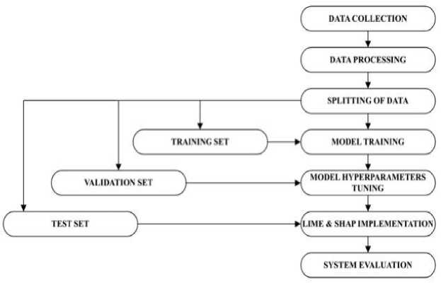
Fig. 1. Methodology of the system

• 3.1    Data Preprocessing

• 3.2    Model Building

• 3.3    LIME Implementation Setup

• 3.4    SHAP Implementation Setup

The loan dataset obtained from Kaggle has 613 columns with key features used in the study, including credit history, applicant income, dependents, loan ID (primary key of the dataset), gender, loan amount, loan term, selfemployed, married, co-applicant income, and education. The preprocessing of the dataset involves handling missing values, removing duplicates, addressing outliers, and standardizing data formats.

Random Forest was used for building the machine learning model because it reduces the risk of overfitting by aggregating predictions from multiple decision trees. It also effectively handles datasets with a large number of features (high-dimensional data) without requiring dimensionality reduction techniques. Random Forest handles imbalanced datasets well, as they are not heavily influenced by the majority class, can capture patterns in the minority class effectively, and provide insights into feature importance. Apart from the Random Forest model having a clearer way of measuring the features’ importance and contribution by reducing uncertainty in making decisions, it is used for explainability tasks because, unlike other models, it provides global interpretability and not just individual predictions. Moreso, Random Forest models typically have higher precision due to their ability to handle non-linearity and interactions between features. Logistic Regression, being linear, on the other hand, may struggle in cases where the decision boundary is complex, which can lower its precision. Support Vector Machine can perform similarly to Random Forest, especially in well-separated classes, but may fall behind when feature interactions become complex. For accuracy, Random Forest performs better because they use multiple decision trees. Random Forest for loan approval systems gives a higher recall, accuracy, and precision when compared with Logistic Regression, SVM achieves precision similar to Random Forest when tuned properly but may require more computational efforts. For the F1 score, Random Forest achieves a high F1 score because of its ability to balance precision and recall compared with other models. The loan dataset is split into training, validation, and testing sets. The training set is used to train machine learning models; the validation set helps tune model hyperparameters; and the testing set is used to evaluate and compare LIME and SHAP explanations.

A loan application instance is selected from the testing set to implement LIME. LIME is used to generate local explanations for the chosen loan application. LIME approximates the behavior of the Random Forest model around the instance of interest by generating a local interpretable model. Next, the features of the loan application are perturbed, and predictions are obtained from the Random Forest model for these perturbed instances. This is followed by fitting a local interpretable model to the perturbed instances and their corresponding model predictions, after which the feature importance values are calculated from the coefficients of the interpretable model. 100 perturbed instances were generated to model the local decision boundary. A linear surrogate model was used with a kernel weight of 0.75. Finally, an explanation highlighting the features and their contributions to the loan approval decision is generated for the selected loan application.

To implement SHAP, the loan application instance used is selected from the same testing set. SHAP is then used to generate explanations for the chosen loan application. TreeSHAP variant was used with 100 background samples randomly selected from the training set with pairwise interaction effects between features. To achieve this, SHAP assigns each feature in the loan application a Shapley value, which represents the average contribution of that feature across all possible feature combinations. Next, the Shapley values for the loan application using the Random Forest model were computed as the machine learning model. An explanation that shows the feature contributions and their impact on the loan approval decision is then generated for the selected loan application. Unlike LIME, SHAP takes into consideration all the loan instances and does not use a single instance to generate an explanation for the prediction.

The primary objective of this comparative analysis is to examine how LIME and SHAP contribute to enhancing the transparency and interpretability of loan approval systems, specifically when combined with the Random Forest machine learning model. The analysis involved implementing both frameworks, generating explanations for loan approval decisions, and evaluating the quality and utility of the explanations. The comparison was conducted using a representative loan dataset obtained from Kaggle with an extract dataset shown in Figure 2.

From the experiment, the system recorded an accuracy of 85%, precision-84%, recall-97%, and an F1 score of 90% for the Random Forest model. A high precision of 84% for this system indicates a low false positive rate, which implies that the risk of granting loans to undeserving borrowers is greatly reduced and there are fewer situations where a customer who ought to be rejected for a loan gets approved. Recall, also known as true positive rate, measures the degree of correctly predicted approved loans out of all actual approved loans. In loan approval systems, recall portrays the model's ability to identify all creditworthy borrowers and avoid false negatives, ensuring that only deserving applicants are approved and not overlooked. A recall of 97% represents a low false negative meaning that the chances

	Loan_ID	Gender	Married	Dependents	Education	SelfEmployed	Applicantincome	Coapplicantincome	LoanAmount	Loan_Amount_Term	Credit_History	PropertyAi
1	LP001003	Male	Yes	1	Graduate	NO	4583	1508.0	128.0	360.0	1.0	Rl
2	LP001005	Male	Yes	0	Graduate	Yes	3000	0.0	66.0	360.0	1.0	Urt
3	LP001006	Male	Yes	0	Not Graduate	No	2583	2358.0	120.0	360 0	1.0	Urt
4	LP001008	Male	No	0	Graduate	NO	6000	0.0	141.0	360.0	1.0	Urt
5	LP001011	Male	Yes	2	Graduate	Yes	5417	4196.0	267.0	360.0	1.0	Urt
609	LP002978	Female	No	0	Graduate	No	2900	0.0	71.0	360.0	1.0	Rl
610	LP002979	Male	Yes	3+	Graduate	No	4106	0.0	40.0	180.0	1.0	Rl
611	LP002983	Male	Yes	1	Graduate	No	8072	240.0	253.0	360.0	1.0	Urt
612	LP002984	Male	Yes	2	Graduate	No	7583	0.0	187.0	360.0	1.0	Urt
613	LP002990	Female	No	0	Graduate	Yes	4583	0.0	133.0	360.0	0.0	Semiurt

Fig. 2. An extract from the dataset

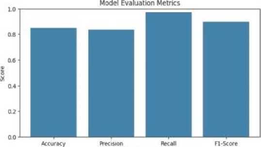
Evaluation Metric

Fig. 3. Random Forest Evaluation Metrics of trustworthy customers being rejected for loans are greatly reduced. F1 score is a combined metric that considers both precision and recall. It provides a balance between these two measures and is particularly useful when the dataset is imbalanced or when both false positives and false negatives need to be minimized. An F1 score of 90% shows the tradeoffs between recall and precision and indicates very low bias in the system explanations in which case the system has low false negatives and low false positives. Comparatively, in terms of interpretability and complexity, these evaluation metrics present LIME and SHAP as very effective explainable AI frameworks in loan approval systems in terms of the explanations and predictions generated.

• 4.1    LIME Explanations

By using LIME, insights can be gained into how the model arrived at a particular loan approval decision for a specific instance. This transparency helps in understanding the reasons behind the decision and detecting any potential biases or discriminatory patterns. LIME explanations can be used to validate and justify individual loan approval decisions by identifying the most influential features for individual loan instances. LIME is designed to be modelagnostic, meaning it can be applied to any machine learning model, including Random Forest, Logistic Regression, or Support Vector Machines (SVM). This flexibility makes LIME suitable for loan approval systems that employ different types of models or when the model used is unknown. It can provide explanations regardless of the underlying model's complexity. Figure 4 displays the LIME explanation for a loan instance highlighting its feature contribution and values. The probability of the loan being approved or not is shown to the left of the figure. In the middle, the most important parameters for the loan being approved (shown in orange) and not approved (shown in blue) are shown. The rightmost part shows the actual values of the parameters. In the context of LIME explanations, the prediction probability of 83% and 17% indicates the likelihood of the loan application being classified as either "NO" or "YES" by the underlying machine learning model. Also as shown in Figure 4, the parameters which increase the possibility of a loan being classified as ‘yes’ are ‘property area’, ‘Gender’, ‘education’, ‘loan amount’, and ‘employment status’ which are ordered by the weights. The features of ‘loan amount term’ (the period the loan is into effect), ‘loan ID’, ‘marital status’, ‘number of dependents’, ‘applicant’s income’, and ‘co-applicant income’ decrease the possibility of the loan being approved. The prediction probabilities represent the probabilities assigned by the local model for each class label, "NO" and "YES" in this case. The given prediction probabilities suggest that based on the features and their contributions identified by LIME, there is a higher likelihood (83%) that the loan application will be classified as "NO" by the underlying model for the given individual given that the explanations are specific to individual instances and provide insights into the factors influencing the prediction outcome.

Prediction probabilities

No ^^HpIbS Yes И 0.17    ~|

No

Loan_Amount_Tcrm >.. 0 .!$■

Yes

0.00 < Propcrty_Area ... l0D6

Married <= 0.00 oosl

Applicantincome <= ...

0.031

Education <= 0.00

l0.03

Dependents <= 0.00 uni

Gender <= 1.00 lOD?

LoanAmount <- 104.00 001

Coapplicantincome <=...

Credit_History <= 1.00

ООО

Self.Employed <= 0.00

DUO

Feature	Value
Loan_Amount_Term480.00 1
	1.00
Loan_ID	168.00
Married	0.00
Education	0.00
Applicantincome	2237.00
Gender	1.00
Dependents	0.00
LoanAmount	63.00
Coapplicantincome	0.00
Self_Employed	0.00
Credit_History	0.00

Fig. 4. A loan approval prediction explained by LIME

• 4.2    SHAP Explanations

• 4.2.1    Summary Plot Explanation

• 4.2.2    Force Plot Explanation

SHAP provides a comprehensive understanding of feature importance, allowing stakeholders to evaluate the influence of different factors on loan approval decisions. This transparency ensures that the decision-making process is not solely based on arbitrary or hidden criteria, but rather on quantifiable and interpretable feature contributions. SHAP values enable stakeholders to assess the relative importance of different features in loan approval decisions by highlighting the relative importance of features at a global level. SHAP requires access to a specific model's internals. It utilizes game theory concepts to attribute the prediction outcome to each feature. This makes SHAP more suitable when the loan approval system uses a specific model, as in this case the Random Forest classifier. SHAP can capture the interactions between features specific to the chosen model, providing detailed insights into the decision-making process. SHAP explanations are provided in four dimensions namely; summary plot, force plots, dependence plot, and interaction plot.

As shown in Figure 5, the y-axis indicates the variable name, in order of importance from top to bottom. The value next to it is the mean on the x-axis showing the SHAP value. For all the features and samples in the selected range, the plot aggregates SHAP values sorted in a way where the most important feature is at the top of the list. The important features of the dataset are shown with the help of a bar diagram, where the features are categorized according to their precedence with credit_history which tops the list having the highest precedence, and self_employed having the lowest precedence at the bottom of the list.

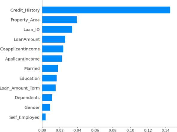
mean(|SHAP value)) (average impact on model output magnitude)

Fig. 5. Bar diagram showing important features of the loan approval dataset

The force plot as shown in Figure 6 indicates the model’s score of 0.74 for the observation. Higher scores lead the model to predict 1 (YES) and lower scores lead the model to predict 0 (NO). The features that were important to predicting this observation are shown in red and blue, with red representing features that pushed the model score higher such as; education, coapplicant income, loan amount, nth term, and the credit_history. While, blue represents features that pushed the score lower such as; gender, marital status, applicant income, property area, and self_employed. The red color typically represents positive contributions, indicating that the feature value increases the prediction compared to the baseline or expected value. Features highlighted in red have a positive impact on the output and contribute to pushing the prediction higher. On the other hand, the blue color represents negative contributions, indicating that the feature value decreases the prediction compared to the baseline or expected value. Features highlighted in blue have a negative impact on the output and contribute to pulling the prediction lower. Features that had more of an impact on the score are located closer to the dividing boundary between red and blue, and the size of that impact is represented by the size of the bar. This particular loan instance was ultimately classified as a yes because they were pushed higher by all the factors shown in red and had a high score of 0.74. The scatter plot shows the different features and the extent of their contributions to the explanation of a given instance.

Prediction probabilities

No ^^И83

Yes #0.17     |

No

Loan_Amount_Tcrm >...

0 15в

Yes

ООО < Property_Arca .., l0J06

LoanJD <= 168.00 onsl

Married <-0.00

0.051

Applicantincome <=... ood

Education <= 0.00

I0j03

Dependents <= 0.00

0.02I

Gender <= 1.00

0 03

LoanAmount <= 104.00 0.01

Coapplicantincome <=...

0.00

Feature	Value
Loan_Amount_Tcrm 480.00 1
Property _Area	1.00
LoanJD Married	168.00 0.00
Education	0.00
Applicantincome	2237.00
Gender	1.00
Dependents	0.00
LoanAmount	63.00
Coapplicantincome	0.00
Self-Employed	0.00
Crcdit_History	0.00

Self_Employed <= 0.00 ало

Credit-History <= 1.00

01)0

Fig. 6. SHAP force plot for a loan instance

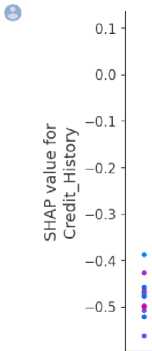
• 4.2.3    Dependence Plot Explanation

The dependence plot in Figure 7 visualizes the relationship between a specific feature and its corresponding SHAP values. In this dependence plot, the feature selected is credit_history. The plot shows how changes in the credit_history feature influence the predicted outcome of the loan approval system. It also helps one to understand the direction and strength of the relationship between the credit_history feature and the loan approval decision. The plot can be interpreted by observing the distribution of points and the trend line. Each dot is a single prediction (row) from the dataset. The x-axis is the value of the feature (credit_history). While, the y-axis is the SHAP value for that feature, which represents how much knowing that feature's value changes the output of the model for that sample's prediction. The color effect corresponds to a second feature that may have an interaction effect with the feature that is plotted (by default this second feature is chosen automatically) in this case, it is the applicant ‘s income. If an interaction effect is present between this other feature and the feature under consideration, it will show up as a distinct vertical pattern of coloring. For instance, the credit history here has no direct interaction with the applicant’s income. However, a sudden loss or reduction in earnings could affect the credit_history indirectly hence, the dependence plot shown.

8000 ш

о

с

6000 з

5000 £

0.0        0.2        0.4        0.6        0.8        1.0

CreditHistory

Fig. 7. Dependence plot for a loan instance.

• 4.2.4    Interaction Plot Explanation

• 4.3    Evaluation & Application

  The explanations were shown to loan officers comprising 10 participants (six males and four females) and their evaluation result shows SHAP generated 10 important features than LIME which generated 8 important features that could aid them in making loan application decisions. It took LIME 0.1486 seconds to generate explanations using 9.14 MB of memory. SHAP used 0.3784 seconds to generate explanations consuming a memory size of 1.2 MB. By demonstrating SHAP's capacity to record feature interactions and offer a more sophisticated comprehension of the relationships between important factors (such as income, credit history, and loan size) in loan approval decisions, the work advances the state of the art. This is important because it helps identify biases or unfair tendencies that more straightforward prediction tools could miss. By directly comparing the computational efficiency of LIME and SHAP, this study makes a novel contribution. It shows that while SHAP's in-depth explanations may be more appropriate for

Finally, the interaction plot shown in Figure 8 visualizes the interactions between different features and their combined effects on the model predictions. In this loan instance, the interaction plot is generated using the SHAP interaction values. This provides insights into how two or more features interact with each other to influence the loan approval decision. The plot displays summary information about the interaction effects across the dataset. Each dot on the plot represents a specific combination of feature values, and its position represents the impact of that combination on the loan approval decision. The color of the dots represents the value of the feature that is being interacted with. It

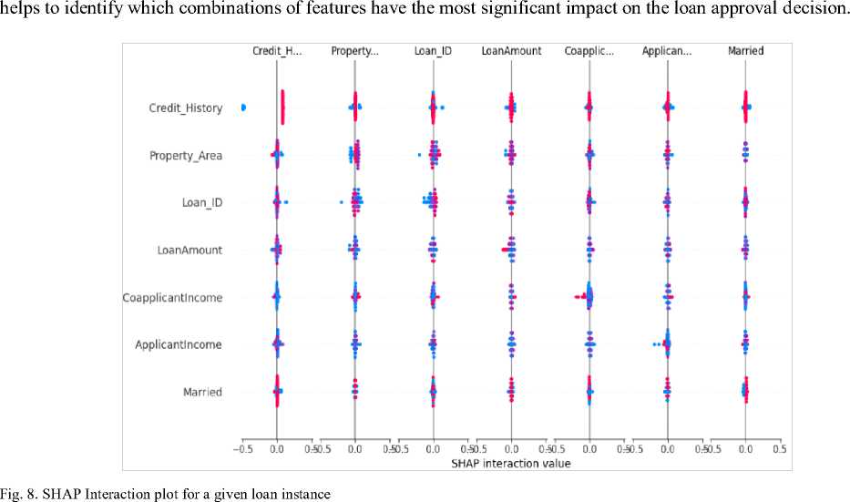
regulatory compliance and auditing tasks, LIME's faster runtime makes it more suitable for real-time loan approval systems. The study also suggests investigating hybrid frameworks that combine the computing power of LIME with the in-depth feature analysis of SHAP, which could result in more reliable and transparent AI systems for financial decision-making. This study acknowledges the possibility that AI algorithms could maintain bias in judgments about loan acceptance. Institutions can identify instances in which sensitive factors (e.g., gender, race) are unfairly influencing model decisions and take corrective action to maintain compliance with fairness rules, such as the Fair Lending Act implemented at some jurisdictions. Explainable AI frameworks help financial institutions, regulatory agencies, and loan applicants to easily comprehend the rationale behind a loan's approval or denial. Their applicants can easily know why their applications are denied and what aspect of their profile needs improvement. Loan officers can verify the AI's judgments, especially in borderline cases, by using the justifications provided by LIME and SHAP. For instance, a loan officer may prioritize credit history when deciding if SHAP indicates that it is the most significant element in the application. Financial organizations can customize loan packages for specific consumers by identifying critical characteristics (such as income and credit history) that impact loan approvals. By highlighting patterns suggestive of fraud or low creditworthiness, LIME and SHAP can assist institutions in optimizing risk evaluations. Loan officers can look into suspicious patterns in real time by analyzing which variables are influencing high-risk judgments.

5    Conclusion

In loan approval systems, the ability to assess the eligibility of individuals and businesses for financial support is of utmost importance. This paper provides a comprehensive comparative analysis of LIME and SHAP within the context of loan approval systems. The analysis evaluated the performance, effectiveness, and interpretability of both XAI frameworks in the context of loan approval systems. The study utilized a loan dataset obtained from Kaggle and implemented LIME and SHAP frameworks to generate explanations for loan approval decisions using the Random Forest model. The results were then discussed and interpreted. Comparatively, LIME provides elaborate insights at the individual instance level while SHAP offers a holistic understanding of feature importance. LIME accommodates different ML approaches compared to SHAP. In terms of interpretability, LIME explanations are simpler and more easily understandable compared to SHAP. SHAP explanations are more complex due to the calculation of Shapley values and the consideration of feature interactions. While they may require a deeper understanding to interpret fully, SHAP explanations reveal hidden connections between features and unveil intricate relationships that contribute to the loan approval decision. The application of LIME and SHAP in loan approval systems has significant implications. It enhances transparency by providing interpretable explanations for individual loan instances and feature contributions, thus enabling stakeholders to understand the decision-making process and detect potential biases. Further research should explore datasets from other sources, as well as other application domains. Advances should also be made in investigating the possibility of combining LIME and SHAP into a hybrid framework that leverages the strength of both techniques.