Comparative analysis of selection and replacement schemes for genetic programming

The genetic programming (GP) approaches are part of evolutionary computation, which is used to create different kinds of program code, starting from relatively simple mathematical equations to complex code with a lot of instructions. There are many GP variants, which have been proposed in the last decades, starting from the simple tree-based GP [1; 2], followed by linear GP (LGP) [3], Cartesian GP (CGP) [4; 5], grammatical evolution (GE) [6; 7] and Push GP [8; 9]. These variants differ in the solution representation, flexibility and capabilities of growing whole programs or parts of programs. These variants of GP are often used as hyper-heuristics to improve existing algorithms automatically, or even create new ones from scratch.

Although GP is a powerful tool to solve many automatic design problems, its main disadvantage is its low computational efficiency conditioned by its huge combinatorial search space. For many years researchers have proposed new selection, crossover and mutation operators, which would improve the efficiency of GP search, and some of them show very promising results. However, most of the used GP frameworks use the same algorithmic structure as a classical genetic algorithm (GA) [10], i. e. a single population, which produces an offspring population, which then replaces its parents keeping an elite individual. This classical scheme is known for its simplicity in implementation and seems to work well.

The focus of this paper is on changing the classical scheme used in most GP variants by changing the selection and replacement schemes. In particular, four selection schemes, two schemes for selecting first parent, and a total of seven replacement schemes are tested in the experiments with a classical tree-based GP on regression problems. The aim of the study is to evaluate the efficiency of different parent and environment selection schemes in genetic programming. The analysis of the experimental results demonstrates that the widely used population management procedures may be suboptimal, and that borrowing some mechanisms from other evolutionary algorithms may be beneficial.

The results show how the genetic programming algorithm can be improved in practice when applied to tasks from various fields, including aerospace. Since the selection mechanisms do not depend on the type of a task, but only on the error values, the proposed GP modifications can be applied to such tasks as predicting the degradation of solar panels, or predicting antenna parameters such as the radiation pattern, including the width of the main and side lobes. For the latter task, a GP for symbolic regression can be used as a surrogate model.

Tree-based genetic programming

A classical tree-based genetic programming was proposed by John Koza in [1]. The idea of this GP consisted in evolving mathematical equations rather than binary strings, as it was in the genetic algorithm. The equations were represented as directed non-cyclic graphs, i.e. trees, where terminal set contained constants and input variables; and functional set contained arithmetic operations (+, -, *, /) and elementary functions (sin, cos, log, exp, …).

The initialization of solutions in GP is performed in a recursive way. First, the type of operation is selected for the starting node. If the operation is binary, two child nodes are created; otherwise, only one is created. Then every child node becomes either functional or terminal. If a node is terminal (leaf node), this branch does not grow further; otherwise, another node is created. There are two main initialization methods, namely full method where leaf node is only placed on a certain maximum depth, and growing method where leaf node can be placed randomly instead of functional nodes.

The selection operators in the classical GP are the same as in GA, as selection does not depend on the solution representation, i.e. the most used approaches are fitness-proportionate selection, rankbased selection and tournament selection [11].

Crossover is one of the most important parts of GP. It creates offspring solutions by exchanging branches between two parent trees chosen by selection. If the branches are chosen randomly, it is called standard crossover. Another method, called one-point crossover, first identifies the common part of two parent trees and then chooses the cutting edge in the common part.

The mutation is also an important part of GP; and there are two main schemes. In the first one, a single node is mutated; therefore it is called point mutation. For example, a binary operation is changed to another binary operation, i.e. + to -, and a constant may be swapped by an input value. Another mutation method is called growing mutation, and it replaces an existing branch or a tree by another one, which is grown in the same way as in the initialization.

The basic classical set of operators described above is commonly used for the tree-based genetic programming in most implementations, although they may vary in some details. Further in this work we will use standard crossover and growing-based mutation.

Lexicase selection and its variants

One of the disadvantages of all classical selection schemes, such as fitness-proportionate, rankbased or tournament, is that they aggregate the quality of an individual into a single fitness value. When dealing with regression, classification or any other type of problems where fitness is composed of quality measures over a set of cases, such aggregation results in loss of valuable information about the performance of a given individual on each particular case. In other words, it is difficult to determine where an individual performs well, and where it does not, if all error values are summed together.

As a solution to this issue, the lexicase selection [12, 13] was proposed, in which the performance e t of all individuals on each training case t in training set T is considered. The main steps of lexicase selection for classification problems are as follows:

• 1.    C:=all individuals i in population P;

• 2.    T’:=randomly shuffled training set T;

• 3.    While |T’|>0 and |C|>1 do

  • 3.1.    t:=first case of T’

  • 3.2.    C:=all candidates with e t =e t *

  • 3.3.    Remove t from T’

• 4.    End while

• 5.    Return random choice from C

Thus, at first all individuals are candidates for selection; and the training set is shuffled. Then cases are taken one by one, and all individuals, which have error values larger than lowest error et*, are fil- tered out. If we run out of cases or candidates, the while loop is stopped. At the end, if there are more than one individual in C, one of them is chosen randomly.

For regression problems and other continuous problems where cases are not only considered to be correctly or incorrectly classified, the ε-lexicase selection was proposed [14, 15]. It modifies the condition in the algorithm by considering the median value as a threshold, i.e. candidates with error e t <=e t *+ε t remain. The threshold value is calculated as ε t =median(|e t -median(e t )|).

In addition to ε-lexicase selection, there are several other variants; some of them implement downsampling strategies. In its simplest form, random down-sampling means that individuals are evaluated not on the whole dataset, but rather on its part, which is randomly sampled from the training set [16, 17]. The sampling is usually repeated every generation. Evaluating on a smaller sample results in a significant speed-up of the whole algorithm, as the lexicase selection is much slower than the tournament of fitness-proportionate. Nevertheless, as the sample is random, it is likely that even with large down-sampling factors d, after several generations every training case will be used.

Proposed approach

In most genetic programming variants and implementation, both parents are chosen for crossover with the currently applied selection mechanism. However, not all evolutionary algorithms follow this scheme. For example, in differential evolution (DE) [18, 19] every individual in the population gets a chance to produce an offspring, i.e. every i-th individual is combined with other ones. This is different from choosing both parents with selection, as there is a chance that some of the individuals will never participate in crossover. The first modification in this work introduces this “give everyone a chance” strategy into GP.

Another important part of every algorithm is the replacement scheme. As mentioned in the introduction, most studies use the simplest mechanism, where parents are replaced by offspring, with keeping the best individual, also known as elitism strategy. However, such a strategy may result in the loss of potentially good solutions, as they may never receive a chance to participate in crossover, as they were never selected and then simply replaced by new ones. In the already mentioned differential evolution, every offspring of every individual is compared to its i-th parent (i=1,2,…N, N is the population size); and the replacement occurs only if the offspring is better. This makes the whole algorithm much more conservative regarding its movement in the combinatorial search space, therefore only positive changes are remembered.

The replacement step can be considered as another selection, where from the joined set of parents and offspring the new population should be selected. One of the simplest alternative approaches here is just to select the best of parents and offspring, i.e. sort them by fitness, and select only first N, where N is the population size. Any other selection mechanism, i.e. tournament selection, rank-based selection and fitness-proportionate selection can be applied here, with the only difference that the same individual should not be selected twice.

Further in this paper the following settings will be considered:

• 1.    Selection mechanisms:

  • 1.1.    Rank-based;

  • 1.2.    Tournament;

  • 1.3.    ε-lexicase;

  • 1.4.    Down-sampled ε-lexicase;

• 2.    First parent selection:

  • 2.1.    Current i-th individual;

  • 2.2.    Same selection as second parent;

• 3.    Replacement scheme:

  • 3.1.    Only offspring with copy of the best individual;

  • 3.2.    Pairwise comparison with i-th parent;

  • 3.3.    Best of parents and offspring;

  • 3.4.    Tournament selection;

  • 3.5.    Rank-based selection;

  • 3.6.    ε-lexicase selection

  • 3.7.    Down-sampled ε-lexicase selection.

This gives a total of 56 different combinations of parameter settings to be tested.

Results

The genetic programming variant used in this study is tree based; and the testing is performed on regression datasets. The datasets have been taken from the Penn Machine Learning Benchmarks (PMLB) [20], in particular, 10 regression datasets have been chosen. Their characteristics are shown in Table 1.

Table 1

Datasets from the PMLB

Dataset name	Instances	Features	Binary features	Continuous features	Categorical features
192_vineyard	52	2	0	0	2
210_cloud	108	5	1	1	3
522_pm10	500	7	0	0	7
557_analcatdata_apnea1	475	3	0	2	1
579_fri_c0_250_5	250	5	0	0	5
606_fri_c2_1000_10	1000	10	0	0	10
650_fri_c0_500_50	500	50	0	0	50
678_visualizing_environmental	111	3	0	0	3
1028_SWD	1000	10	1	9	0
1089_USCrime	47	13	1	0	12

The GP had the following settings. The set of operations included: +, -, *, /, ln, exp, sqrt, sin, cos, tan, tanh, 1/x, sinh, cosh, abs. If some operation yielded NaN or very big number, it was replaced by a numeric limit, set in the C++ language for double data type. Only standard crossover and growing mutation were used. Other numeric parameters are below:

• 1.    Population size N=100;

• 2.    Maximum depth at initialization: MaxD=5;

• 3.    Probability to end branch during initialization InitProb=0.1;

• 4.    Constant generation: with Cauchy distribution, scale parameter=5, location parameter equals last constant value;

• 5.    Tournament size T=3;

• 6.    Rank-based selection with exponential ranking and parameter k=3;

• 7.    Maximum number of nodes in a tree: MaxL=75;

• 8.    Computational resource: NFEmax=100000 evaluations;

• 9.    Down-sampling factor d=5;

• 10.    Number of runs on each dataset NR=25;

• 11.    Fitness measure: coefficient of determination R2.

44

1.4

2.1

3.2

0–/10=/0+

–2.79

39.72

45

1.4

2.1

3.3

0–/10=/0+

0.00

34.08

46

1.4

2.1

3.4

10–/0=/0+

–34.46

235.60

47

1.4

2.1

3.5

10–/0=/0+

–34.11

239.08

48

1.4

2.1

3.6

10–/0=/0+

–33.49

228.68

49

1.4

2.1

3.7

10–/0=/0+

–33.66

231.04

50

1.4

2.2

3.1

8–/2=/0+

–29.41

169.08

51

1.4

2.2

3.2

0–/10=/0+

–19.44

94.20

52

1.4

2.2

3.3

0–/10=/0+

–3.63

44.28

53

1.4

2.2

3.4

10–/0=/0+

–33.86

232.62

54

1.4

2.2

3.5

10–/0=/0+

–34.38

232.60

55

1.4

2.2

3.6

10–/0=/0+

–32.81

227.44

56

1.4

2.2

3.7

10–/0=/0+

–33.66

224.80

The genetic programming was implemented in C++, compiled with GCC, and ran on an OpenMPI-powered cluster on 16 computers under Ubuntu 20.04 with AMD Ryzen 5700X processors, each with 8 cores and 16 threads. The post-processing of results was performed in Python.

To compare the results of runs with different parameters, two instruments were used, namely the Mann-Whitney statistical test for pairwise comparison of algorithms, and Friedman ranking procedure to compare all the results. The Friedman ranking procedure is taken from the Friedman statistical test, and it ranks all runs of all configurations on a single function independently, and then these ranks are summed together. Table 2 contains the comparison where the notation of selection, first parent choice and replacement follows the numbering in the previous section (for example, tournament replacement is 3.4). The Mann-Whitney tests (denoted as M-W) were performed for every dataset independently, and the number of losses/ties/wins are shown as x-/y=/z+. The total Z-score is calculated as the sum of Z-distributed values, which were used in the normal approximation of the Mann-Whitney U statistics. The significance level threshold was set to p=0.01. In Table 2 the run with number 45 was chosen as baseline as it demonstrated the best results (down-sampled ε-lexicase, current i-th individual, pairwise comparison with i-th parent).

Comparison of the 56 tested algorithm configurations

Table 2

#	Selection	First parent	Replacement	M-W test	Z-score	Friedman rank
1	1.1	2.1	3.1	10–/0=/0+	–43.64	389.16
2	1.1	2.1	3.2	0–/10=/0+	–19.01	160.32
3	1.1	2.1	3.3	1–/9=/0+	–16.47	134.44
4	1.1	2.1	3.4	10–/0=/0+	–45.33	433.96
5	1.1	2.1	3.5	10–/0=/0+	–45.67	445.88
6	1.1	2.1	3.6	10–/0=/0+	–46.22	446.72
7	1.1	2.1	3.7	10–/0=/0+	–33.61	227.16
8	1.1	2.2	3.1	10–/0=/0+	–42.05	376.88
9	1.1	2.2	3.2	9–/1=/0+	–30.50	226.92
10	1.1	2.2	3.3	1–/9=/0+	–19.42	157.12
11	1.1	2.2	3.4	10–/0=/0+	–45.73	443.32
12	1.1	2.2	3.5	10–/0=/0+	–46.22	452.92
13	1.1	2.2	3.6	10–/0=/0+	–45.91	442.78
14	1.1	2.2	3.7	10–/0=/0+	–34.56	241.08
15	1.2	2.1	3.1	10–/0=/0+	–39.95	343.92
16	1.2	2.1	3.2	0–/10=/0+	–16.10	135.72
17	1.2	2.1	3.3	0–/10=/0+	–14.36	123.28
18	1.2	2.1	3.4	10–/0=/0+	–46.12	443.20
19	1.2	2.1	3.5	10–/0=/0+	–45.93	449.36
20	1.2	2.1	3.6	10–/0=/0+	–45.93	443.46
21	1.2	2.1	3.7	10–/0=/0+	–33.74	232.56
22	1.2	2.2	3.1	10–/0=/0+	–40.94	345.80
23	1.2	2.2	3.2	9–/1=/0+	–30.48	230.80
24	1.2	2.2	3.3	3–/7=/0+	–23.26	179.36
25	1.2	2.2	3.4	10–/0=/0+	–45.23	436.36
26	1.2	2.2	3.5	10–/0=/0+	–45.60	440.52
27	1.2	2.2	3.6	10–/0=/0+	–45.73	445.72
28	1.2	2.2	3.7	10–/0=/0+	–34.19	234.94
29	1.3	2.1	3.1	10–/0=/0+	–38.59	339.08
30	1.3	2.1	3.2	0–/10=/0+	–15.60	134.32
31	1.3	2.1	3.3	0–/10=/0+	–12.44	106.72
32	1.3	2.1	3.4	10–/0=/0+	–45.87	446.56
33	1.3	2.1	3.5	10–/0=/0+	–45.40	439.80
34	1.3	2.1	3.6	10–/0=/0+	–47.15	457.00
35	1.3	2.1	3.7	10–/0=/0+	–33.39	238.92
36	1.3	2.2	3.1	10–/0=/0+	–41.44	380.08
37	1.3	2.2	3.2	10–/0=/0+	–36.57	276.88
38	1.3	2.2	3.3	0–/10=/0+	–15.81	131.16
39	1.3	2.2	3.4	10–/0=/0+	–45.77	436.08
40	1.3	2.2	3.5	10–/0=/0+	–45.50	441.60
41	1.3	2.2	3.6	10–/0=/0+	–45.98	437.76
42	1.3	2.2	3.7	10–/0=/0+	–34.15	231.88
43	1.4	2.1	3.1	8–/2=/0+	–28.62	165.28

Discussion of results

The three best parameters combinations in Table are highlighted in gray, namely combinations 44, 45 and 52. As can be seen, all of them have the same selection mechanism – down-sampled ε-lexicase selection; and all other variants have much lower performance. As for the first parent selection, two out of three best variants used the choice of i-th individual, giving each of them a chance to produce offspring. Finally, the replacement scheme in best variants is either pairwise comparison with i-th parent, or best of parents and offspring.

In other words, these results show that the genetic programming performs much better if the typical algorithmic structure changed to the one used in differential evolution. To compare other operators between themselves, in Fig. 1 the bar plots of total Friedman ranks for every type of selection, first parent choice and replacement are shown.

Total Friedman rank

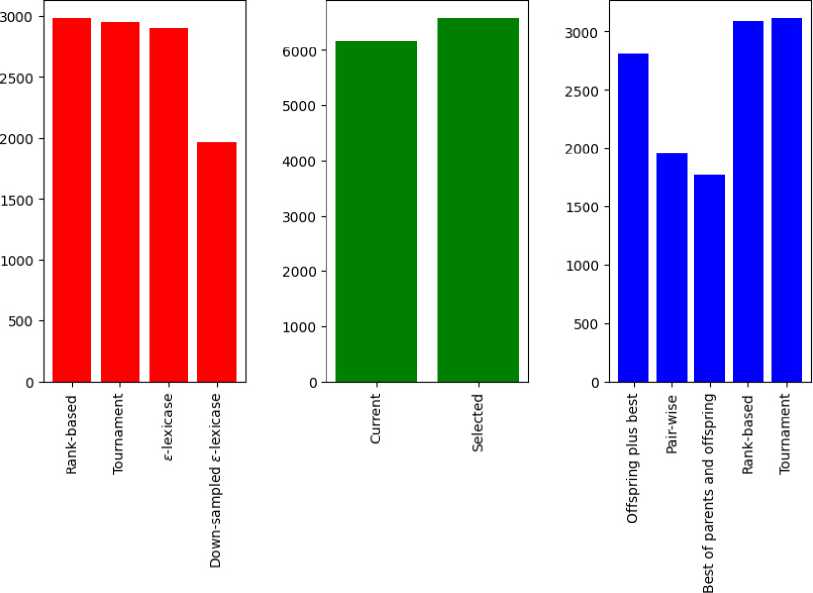
Рис. 1. Столбчатая диаграмма сумм рангов по Фридману для всех типов протестированных операторов

Fig. 1. Bar plot of sums of Friedman ranks for all types of tested operators

As Fig. 1 shows, there is not much difference between the performance of rank-based, tournament and ε-lexicase selection overall; however, the down-sampled ε-lexicase selection performs much better. As for the selection of the first parent, there is a difference between the classical scheme, where it is chosen with the currently used selection operator, and the choice by index. The replacement schemes seem to be very different, and significantly influence the final performance. In particular, “the best of parents and offspring” significantly outperforms all other methods followed by pair-wise comparison. The down-sampled ε-lexicase selection performs better than the rest of the methods, and the widely used offspring plus copy of best parent is significantly worse.

To better understand the reasons why certain replacement schemes work better, in Figure 2 the example is shown where the first two columns are the population and their offspring, with fitness shown in colors (smaller is better), and the other four are the results of different replacement mechanisms. As can be seen, the best of parents and offspring called “elite” for short, simply copies all the offspring, and replaces one of them with the best parent. This results in rapid change of generations, but may lead to the loss of good solutions. The pairwise comparison, on the other hand, keeps the best version of each solution from the population and the offspring, leading to a more stable, although slow progress.

Population Offspring Elite Pairwise

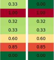
Рис. 2. Пример работы стратегий замещения

Sort Tournament

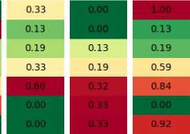
Рис. 2. Example of replacement strategies operation

The sorting simply takes the best individuals from both, and discards all the rest – as the experiments have shown, it is usually a very efficient strategy. The last column shows the tournament selection, but other ones, such as rank-based or lexicase, will have a similar picture. As can be seen, the tournament selection may sometimes select bad solutions and miss the best ones, resulting in subopti-mal progress.

Conclusion

The experiments performed in this work have shown that the typically used population management scheme in genetic programming is suboptimal. The replacement procedure plays a crucial role in algorithm performance, and it is often overlooked by many researchers. The usage of simple strategies, such as pair-wise comparison, combined with the selection of first parent as current i-th individual gives significant performance improvement to the genetic programming algorithm.

However, there are several limitations regarding this study. Here the focus was only on solving regression tasks; and other types of problems, such as regression, control or program synthesis, were not tested. Nevertheless, it is expected that similar trends should be observed for other problem classes, as selection does not depend on the type of problem being solved – it only relies on the error values, but this should be carefully tested in further research.