Comparative analysis of univariate forecasting techniques for industrial natural gas consumption

Published Online May 2018 in MECS DOI: 10.5815/ijigsp.2018.05.04

Forecasting is the process of making future predictions based on past and present data and most commonly by analysis of trends[1]. It has applications in a wide range of fields where estimates for future are useful like product forecasting, sales forecasting, flood forecasting, electricity forecasting, natural gas forecasting etc. There is a continuous rise in the requirement of energy demand worldwide, this includes electricity, coal, natural gas or any other form of energy. According to [2] world consumption of natural gas increases by 1.7% annually for industrial use and the annual rise in consumption of natural gas is 2.2% for the electric power sector. The total share of both industrial and electric power sectors contribute to 73% of the total increase in world’s natural gas consumption, and they expected to rise this to about 74% of total natural gas consumption by 2040.

This paper attempt to evaluate the precise forecast of existing univariate forecasting techniques by providing accurate and statistically significant forecasts for natural gas consumption at the organization level. Various time series based forecasting techniques like Naïve method, Drift method, Simple Exponential Smoothing (SES), Holt method, Holt method with drift, ETS(Error, trend, seasonal) method, ARIMA and Feedforward Neural Network are analyzed.

This paper reports the results from the seven most competitive forecasting techniques. Comparison between these methods is performed by error analysis and time series cross-validation by taking the forecasting horizon of one and three months ahead. On comparison of univariate models used in this article, we find that ARIMA model provides most promising results for the particular dataset under consideration.

• II.    Related Work

The Naïve method represents predicted values as the last observed value in the time series. Drift method represents the amount of average change over time on past values. This change can be decreasing or increasing. All these methods i.e. Naïve and Drift are available as established standard methods of forecasting. A new method of forecasting can be compared with these established methods and its performance can be evaluated [6].

Exponential smoothing method has been around since the 1950s and is the most popular forecasting method used in business and industry [7]. In reference [8] the analysis of seasonal time series data using Holt-Winters exponential smoothing method is being produced with a discussion of multiplicative seasonal model sand additive seasonal models. In reference[9], formulae are given for evaluating mean and variances for lead time demand of exponential smoothing method over a wide range. In reference[10] researcher provided forecasting of inventory control using exponential smoothing.

The Holt-Winters forecasting procedure is a variant of exponential smoothing and suitable for producing shortterm forecasts for sales or demand time-series data [11]. In reference [12] long lead-time forecasting by HoltWinters method for UK air passengers is available. Reference [13] describe Holt-Winters method with different models of forecasting and prediction intervals for the multiplicative model.

In reference [22] researcher explain transit containers in Kaohsiung port by adopting artificial neural network(ANN).In reference [23] a model of neural networks (NN) for forecasting throughput of Hong Kong port cargo has been discussed. Reference [24] used the NN approach to forecast time series on a quarterly basis.Reference [25] and [26] applied error correction model to forecast Hong Kong’s throughput. Reference [27] describe ANN with seven different algorithms, namely-Limited Memory Quasi-Newton Algorithm, Conjugate Gradient Descent Algorithm, Quasi-Newton Algorithm, Levenberg-Marquardt Algorithm, Quick propagation Algorithm, Incremental Back-Propagation Algorithm and Batch Back-Propagation Algorithm to achieve daily and monthly forecast of natural gas consumption in Istanbul. Reference [28] describe Artificial Neural Networkandartificial bee colony (ABC) algorithm to study consumption demand forecasting on monthly basis. In Reference [40] Artificial Neural Network (ANN) technique has been used to develop onemonth and two month ahead forecasting models for rainfall prediction using monthly rainfall data of Northern India. A Neural Network structure has been used to forecast the stock values of different organizations of Banking and Financial sectors in NIFTY 50 [41].

• III.    Methodology

In this section, we presented the details about all the univariate forecasting models considered for natural gas consumption forecasting. Consideringy 1 , y 2 ,  y T represents previous data. У т+hiT represent forecasted values based upon y ₁ , y ₂ ,   y _T, the various techniques of forecasting are as discussed below:

• A.    Univariate Forecasting Techniques

• 1)    Naïve Method

In this method, forecast value is equal to last measured value. If y T is the last measured value of time series data then future values represent the same value [29, 30].As naive method provides information about the most recent values, the forecast value generated from the Naive model is not linked with previous values present in Time series [29, 30].

Forecasts Equation:

У т+hlT = У т                 (1)

• 2)    Drift Method

In Drift method, forecast value is the sum of last measured value and the average change in time series. This method allows a change in forecast values to increase and decrease over time depending upon the average change within the time series.

Forecasts Equation:

• У т+hiT = У т ⁺^ ^- ^T t=^_t - y t-1 )

= y_r ⁺ ^" (У т ^- У 1 )           (2)

• 3)    Simple Exponential Smoothening Method

Forecasts values generated are weighted averages of past observations, with the weights decaying exponentially as the observations get older. The value of α falls between zero and unity, the pattern of weights attached to the observations shows exponentially decreasing trend. The value of α towards zero indicates more weight of observations of long past. However larger values of α towards one signifies more weight to recent observations [29, 30].

Forecast equation :

y t+h|t = Z j=1 а ⁽ 1 - a^{)t -j} y j⁽ 1 - a) i o , Where (0 <  а > 1)                (3)

ɩ t is an unobserved “state”.

• 4)    Holt's Method

Holt makes an extension to Simple exponential smoothing method to allow forecasting of data with trends. Two smoothing parameters are being introduced namely: αand β [29, 30].

Forecast Equation:

y t+hit = I t + hb_t

Level      I t = ay t + (1 - a Xl_t -1 + b_t -1 )

Trend     b t = P*(l t — l t-i ) + (1- /? * )b t-i     (4)

l_t indicatethe estimate of level of the series at time t. b_t indicatethe estimate of the slope of the series at time t.

• 5)    ETS Method

Each model has equations for states level, trend and season. It is also known as state space models [29, 30]. Two models for each method: namely additive and multiplicative errors. A combination of 30 models is found. Additive and multiplicative methods provide the similar point forecasts with different forecasting intervals.

ETS(Error, Trend, Seasonal):

– Error={A,M}

– Trend ={N,A,A d ,M,M d }

– Seasonal ={N,A,M}.

ETS (M,A,N)

^yt = ^(lt-i ^{+ b}t-i^{)(1 +} ^ t ) ^lt = ^(lt-i ^{+ b}t-i^{)(1 + a} £ t )

b t = b t-i + P(l t-i + b t-i )£ t          (5)

In this model error is multiplicative, the trend is additive and no season is available.

• 6)    ARIMA Method

For any given time series of data Xt, the ARMA model is a technique for predicting future values in the given time series. The model has two components, first is autoregressive (AR) and another is moving average (MA) part. The AR components include regressing the variable on its own lagged or past values. The MA part includes modeling the error term as a linear combination of error terms. An autoregressive integrated moving-average(ARIMA) model is a generalization of an autoregressive moving average (ARMA) model.In ARIMA differencing is performed to make time series stationary[31, 32].

for zero differencing xt = Xt for differencing only once xt = Xt - Xt-1

And the general equation is given as

• ^Xt = c + 1 ^=1 ⁽Pi^xt-i ^- 1 ^=1⁶i^et-i        ⁽⁶⁾

where the moving average term is negative as the error is minimized each time differencing is done.

• 7)    Neural Network

It is a class of statistical methods for information processing consisting of a large number of simple processing units (neurons), which exchange information of their activation via directed connections[33, 34, 35].

Activation Function

Г¹     if IjWjiXj ^- 0i

( 0 if T,j WjiXj - 0i

Where y_i is output function, x_i is input and w j _i represents the intermediate nodes.

• B.    Accuracy measures

Any forecasting technique needs to be evaluated for prediction accuracy. Accuracy measures check the errors between obtained values and actual values during prediction. Let y t denote the t^th observation and y't\t- ₁ indicate its forecasted value based on previous values, where t =1,...,T. The following measures are used to measure the accuracy of forecasting method. Mean absolute error (MAE) is the average absolute error value. The effectiveness of forecast is considered good for the value of MAE close to zero. Mean squared error is defined as the sum or average of the squared error values[48]. MAE (“Eq. (8)”),    MSE(“Eq. (9)”),

RMSE(“Eq. (10)”) are all scale dependent. MAPE (“Eq. (11)”) is scale independent but is only sensible if y_t >> 0 for all t, and y has a natural zero [36]. The formulas for errors are as follows:

MAE = T-1XT=ilyt-ytit-i I(8)

MSE = T-1TJt=i(yt-ytit-i)2(9)

RMSE= Jt-1 ZT=1( yt-ytit-1)2(10)

MAPE = 100T-1 YT-i |yt-lj>t|lt"1|(11)

L 1

Along with the accuracy measures, Akaike information criterion(AIC) represents the criteria to select the appropriate model."AIC" is an estimate of a constant plus the relative distance between the unknown true likelihood function of the data and the fitted likelihood function of the model. Lower AIC means a model is considered to be closer to the truth [37-38].

• C.    Time series cross-validation

In time series cross-validation [39], many different training sets, each containing one more observation than the previous one are used. Assuming that there is a requirement of k observations for producing a strong reliable forecast, the process can be described as below steps.

• 1.    Pick the test set observation for time t= k + i and use the observations at times 1,2,...,k + i - 1 to estimate the forecasting model. Calculate the error on the forecast for time k + i.

• 2.    Repeat the above step for i = 1,2,..., T - k where T is the overall number of observations.

• 3.    Based on the errors evaluated, calculate forecast accuracy measures.

• D.    Proposed Framework

To perform a comparative analysis, first data collection is carried out. The forecasting techniques (Naïve, Drift, SES, Holt method, ETS, ARIMA, and Neural network) have been applied to collected data and forecasted values have been obtained for each technique. The error components RMSE, MAE, MAPE, and MASE have been worked out for each forecasting technique. Time series

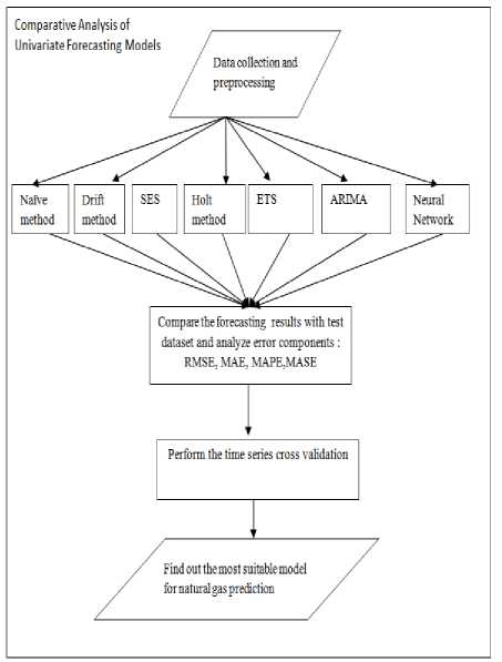
Fig.1. Framework for comparison of Univariate Forecasting Models cross-validation is also performed for various forecasting techniques. The complete framework for forecasting of the univariate model is shown in figure-1.

• IV.    Experiment and Result

This section is divided into three parts. The first section describes the data related to industrial natural gas consumption, second will show the results from different forecasting techniques and third contains the crossvalidation and error analysis to check the most suitable forecasting techniques for this natural gas data.

• A.    Industrial natural gas monthly consumption data

  A monthly dataset is prepared by collecting natural gas consumption data from CFFP, a manufacturing unit of Bharat Heavy Electricals Limited, India for their consumption of natural gas production of Castings products from year April 2014 to January 2017. The consumption data is measured in scm (standard cubic meter) for this period. This is the total sum of consumed natural gas in all the operations related to the casting process. In order to examine the pattern and behavior of data with respect to time, a time series plot of considered data has been drawn in figure 2.

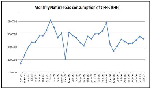
Fig.2. Monthly natural gas consumption in CFFP,BHEL

To perform the forecast of natural gas consumption on monthly basis for CFFP, BHEL, various univariate forecasting models have been implemented and their comparative analysis is done. This study identifies the most suitable model for short-term forecasting on the basis of error analysis for 1- month forecast, and 3-month forecast. For any forecasting method, forecasting period should be predefined that requires the division of data in two parts i.e. in sample period and out-of-sample period. The dataset used for identifying the relationship between the data is termed as training set or in-sample period. On the other hand, test set or out-sample period is the data set that is used to examine the strength of the predicted relationship.

• 1.    Training set: Month1 to Month 30 used for model development.

• 2.    Test set: Month 31 to Month 34 used for training Purpose.

To further analyze the randomness of the considered data, autocorrelation (ACF) plot as shown in figure 3 was created. This is used to measure the relationship between lagged values of time series. At lag 1 the value is significant, representing the strong correlation between successive values .

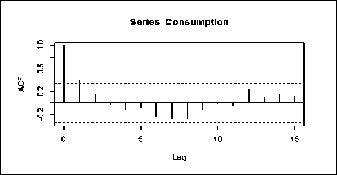
Fig.3. Autocorrelation Plot

• B.    Results from forecasting Techniques

This section contains the details of all fitted model for 1- month forecast of natural gas consumption. The forecast values are generated from the Random walk, SES, Holt, ETS, ARIMA and Neural Network.

• 1)    Naïve method (Random Walk) Method

Naïve or random walk method is the most basic method for forecasting. The Forecasted values generated from this method is equal to the last observed value i.e. in our training set, we consider 1 to 30 months data than for 1- point forecast 31th observation will represent forecasted value. Figure 4 and Figure 5 are the graphical representation of forecasted values from a naïve random walk with drift method respectively. Table 1 represents both of these forecasted values. Random Walk with drift method provides forecast values equal to the sum of final observed value and average change in time series.

Table 1. Forecasted Values from Random Walk Method

S. No.	Test set	Naïve	Drift
1	1653243	1625847	1652319

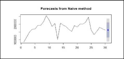
Fig.4. 1-Month ahead Forecast from Random Walk/Naïve method

Forecasts from Random walk with drift

0       5      10      15      20      25      30

Fig.5. 1-Month ahead forecast from Random Walk with Drift method

• 2)    Simple Exponential SmoothingMethod

Forecast with Simple Exponential Smoothing (SES) method requires initialization of smoothing parameter. In SES only one parameter, alpha, is used for Smoothing. The parameters alpha has values between 0 and 1. If the value is close to 0 it represents that less weight is assigned to a most recent measured value. The estimated value of alpha for 1- month natural gas consumption forecast is 0.61. This represents the current value relation with last measured value. Table 2 depicts forecasted value from SES. Figure 6 shows the forecasted value from SES graphically and figure 7 is also graphical representation for level decomposition by SES method.

Table 2. Forecasted Value from SES Method

S. No.	Test set	SES
1	1653243	1666915

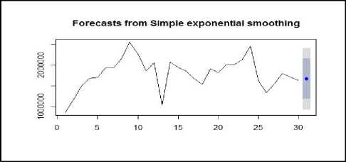
Fig.6. 1-Month ahead Forecast from SES method

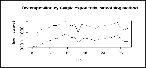
Fig.7. Decomposition from SES method

• 3)    Holt's Method

  The smoothing parameters for Holt’s method are denoted by α and β with values ranging from 0 to 1. For 1-month ahead, forecast of natural gas consumption has α = 0.6014 andβ = 0.0733. Damped Holt's method has smoothing parameter with one damping parameter ϕ, with constraint 0<ϕ<1. For 1-month forecast of natural gas consumptionα = 0.4473,β = 0.0001 and ϕ = 0.8588. Figure-8and figure-9 graphically represents the forecasted values from Holt’s method and Damped Holt’s method with drift respectively. Table 3 represents both the forecasted values.

Table 3. Forecasted Values from Holt's Method

S. No.	Test set	Holt	Damped Holt
1	1653243	1634483	1674545

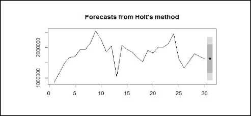
Fig.8. 1-Month ahead Forecast from Holt's method

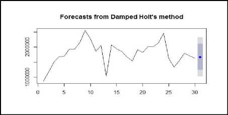
Fig.9. 1-Month ahead Forecast from Holt's with Damped method

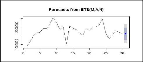
Fig.10. 1-Month ahead Forecast from ETS method

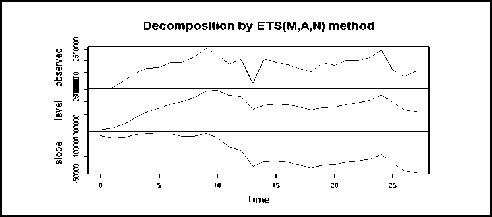
Fig.11. Decomposition from ETS method

• 5)    ARIMA Method

The forecast with ARIMA is done using Hyndman-Khandakar algorithm that minimizes AIC values to arrive at an appropriate model with p, d, and q parameter. It performs changes in p and q values by a maximum of ± 1. ARIMA model selected for1-month forecast is of the order ARIMA(1,0,0). In which p=1, represent AutoRegressive (AR) component of the first order. The value of d define the order of differencing, here d=0 represent series is stationary and auto-correlated. The q=0 shows the absence of Moving Average term. Table 5 depicts forecasted value from ARIMA method. Figure 12isgraphical representation of the forecasted value from ARIMA method.

ETS method for this forecast contains multiplicative level, additive trend, and absence of seasonal component given by N. The Smoothing parameters of fitted ETS (M,A,N) model are α = 0.4486 and β= 0.0648. Table 4 represents a forecasted value from ETS method. Figure 10 graphically shows the forecasted value from ETS and Figure 11 is graphical representation for level decomposition by ETS method.

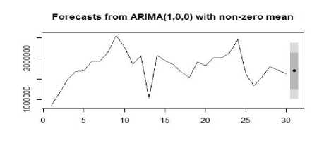
Fig.12. 1-Month ahead Forecast from ARIMA method

Table 4. Forecasted Value from ETS Method

S. No.	Test set	ETS(M,A,N)
1	1653243	1620304

Table 5. Forecasted Value from ARIMA Method

S. No.	Test set	ARIMA (1,0,0)
1	1653243	1695431

• 6)    Neural Network

This forecast uses feed-forward networks denoted by NNAR(p,k) to indicate that there are p lagged inputs and k nodes in the hidden layer. Fitted neural network NNAR(1,1) model denotes one input layer, one hidden layer, and one output layer. The value p=1 tells that only previous value act as input to the model. The value of k represents that only single neuron is present at hidden layer. The generated model is the average of 20 networks, each of which is a 1-1-1 network with linear output units. In table 6 forecasted value from Neural Network method is presented. Figure 13 shows a graphical representation of the forecasted value from Neural Network method.

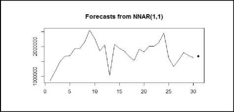
Fig.13. 1-Month ahead Forecast from Neural-Network method

Similarly, forecast values generated for the 3-month forecast for the training set 1 is represented in figure 14.

Table 6. Forecasted Value from Neural Network Method

S. No.	Test set	Neural Network
1	1653243	1678049

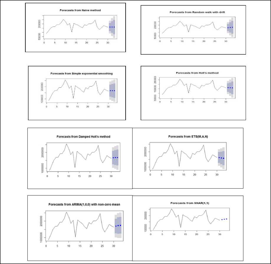
Fig.14. 3-Month Forecast values from Different Models for training set 1

• C. Cross-validation and Error Analysis

In time series cross-validation, the procedure for validation is to use different training sets, each one containing one more observation than the previous one.

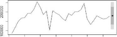
In our 1 -month forecast we start with 30 months data as a training set and predict for 31stmonth value. In the next step, the value of training set has been incremented by one i.e. now 31 values are there in training set and prediction is made for 32nd-month value. Similarly, we move to the 3rd and 4th step. Figure 15defines the procedure for time series cross-validation where blue dots represent training set, red dot represent test data and black dot is not considered in forecasting. In 3 -month forecast we start with 30 months data as a training set and predict for three points ahead i.e. 31th, 32nd and 33rd-month value. In the next step, the value of training set has been incremented by one i.e. now 31 values are there in training set and prediction is made for next three months value explained in figure 16.

Training Set                                       Test Set

Stepl: O-O-O-O-O-O-O-O-O-O-O-O-O-O-O-O-O-O-O-O-O-O-O-O-O-O-O-O-O-C-l-O-O-O

Step 2: O-O-O-O-O-O-O-O-O-O-O-O-O-O-O-O-O-O-O-O-O-O-O-O-O-O-O-O-O-O-O-l-O-O

Step3: 0-0-0-0-0-0-0-0-0-0-0-0-0-0-0-0-0-0-0-0-0-0-0-0-0-0-0-0-0-0-0-0-|-0

Step 4: O-O-O-O-O-O-O-O-O-O-O-O-O-O-O-O-O-O-O-O-O-O-O-O-O-O-O-O-O-O-O-O-i |

• Fig.15.    Time-Series Cross-validation for 1-month forecast

Training Set                             Test Set8ф1:«ШШШШМШ»ММ»ММ«|||<

$фШШШЖиОМт1ЖМ-М»М|||

• Fig.16.    Time-Series Cross-validation for 3-month forecast

All these steps have been performed using all the method defined in section III. The forecasted values are generated from these methods with the different training set for 1-month and 3-month forecast. Table 7 summaries obtained forecast values at each step.

Tr1, Tr2, Tr3, and Tr4 are the four training set for the different step of cross-validation. We check the accuracy of each model using AIC parameter of chosen techniques that are shown in table 8. The AIC value for 1-month forecast for all four training sets Tr1, Tr2, Tr3, and Tr4 are 854.83, 882.11, 909.39, 936.78 respectively for ARIMA technique. It is clear from table 8 that these AIC values for ARIMA are lowest as compared to all other forecasting techniques. Similar findings are observed and recorded for 3-month forecast as shown in table 8. Therefore this cross-validation established that ARIMA (1,0,0)is the most suitable forecasting technique for such time series data.

Table 7. Forecasted Values from Different Models

1-Month ahead Forecast
Traini ng set	Test set	Naïve	Drift	SES	Holt	Holt Damp ed	ETS	ARIM A (1,0,0)	Neural Netwo rk
Tr1	16532 43	16258 47	16523 19	16669 15	16344 83	16745 45	16203 04	16954 31	16780 49
Tr2	17708 41	16532 43	16797 46	16601 74	16321 18	16661 28	16138 35	17068 92	16900 50
Tr3	19077 09	17708 41	18002 83	17259 34	17141 68	17139 81	17205 85	17659 97	17861 47
Tr4	18203 79	19077 09	19405 08	18384 49	18472 84	18022 69	18046 14	18361 23	19043 73
3-Month ahead Forecast
Traini ng set	Test set	Naïve	Drift	SES	Holt	Holt Damp ed	ETS	ARIM A (1,0,0)	Neural Netwo rk
Tr1	16532 43	16258 47	16523 19	16669 15	16344 83	16745 45	16203 04	16954 31	16780 37
	17708 41	16258 47	16787 92	16669 15	16191 56	16757 57	15965 56	17290 28	17089 32
	19077 09	16258 47	17052 64	16669 15	16038 24	16767 97	15728 08	17452 49	17307 39
Tr2	17708 41	16532 43	16797 46	16601 74	16321 18	16661 28	16138 35	17068 92	16900 51
	19077 09	16532 43	17062 49	16601 74	16183 24	16671 62	15923 44	17329 53	17139 07
	18203 79	16532 43	17327 52	16601 74	16045 31	16680 49	15708 53	17456 14	17314 34

Table 8. AIC Parameters for Different Model

Method	AIC for 1-month forecast				AIC for 3-month forecast
	Tr1	Tr2	Tr3	Tr4	Tr1	Tr2
SES	879.044	908.143	932.6278	961.8721	879.0435	908.1429
Holt	880.661	909.686	938.8584	968.1831	880.661	909.6857
Holt Damped	877.451	906.304	935.2558	964.4701	877.4514	906.304
ETS	872.505	901.006	928.7165	957.7302	872.5053	901.0062
ARIMA	854.83	882.11	909.39	936.78	854.83	882.11

Furthermore, the analysis of different types of errors occur during forecasting at each step of validation is performed. To compare the accuracy of various models the average value is evaluated. Table 9 represents the error components occur during forecasting from different models. Now we plot the error terms from each model into a single plot. Figure 17 and 18 depicts the error terms for each model and it is clear that all the concerned error components have minimum values for ARIMA method in comparison to other methods. Thus, it is concluded that ARIMA (1,0,0) is good techniques to forecast for the available training and test data set.

Table 9. Error Components for 1-Month and 3- Month Forecast

Method	Errors	Errors for 1-month Forecast					Errors for 3-month forecast
		Tr1	Tr2	Tr3	Tr4	Average	Tr1	Tr2	Average
Naïve	RMSE	27396	117598	136868	87330	92298	183684.5	188429.2	186056.85
	MAE	27396	117598	136868	87330	92298	151417.3	179733.3	165575.3
	MAPE	1.657107	6.640799	7.174469	4.797353	5.067432	8.206621	9.720337	8.963479
	MASE	0.098576	0.436246	0.517135	0.335018	0.346744	0.544826	0.666745	0.605785
Drift	RMSE	923.6897	91094.9	107426.4	120128.7	79893.4224	128397.8	137310.8	132854.3
	MAE	923.6897	91094.9	107426.4	120128.7	79893.4224	98472.71	126727.1	112599.91
	MAPE	0.05587138	5.14416	5.631171	6.599105	4.35757684	5.288626	6.839371	6.0639985
	MASE	0.003324	0.337929	0.405894	0.460842	0.301997	0.354322	0.470112	0.412217
SES	RMSE	13672.19	110666.9	181774.9	18070.08	81046.0175	151623.6	181829.9	166726.75
	MAE	13672.19	110666.9	181774.9	18070.08	81046.0175	119463.9	172802.3	146133.1
	MAPE	0.8269921	6.2494	9.528439	0.992655	4.39937152	6.439288	9.341848	7.890568
	MASE	0.049195	0.410534	0.686809	0.069321	0.303965	0.429852	0.641034	0.535443
Holt	RMSE	18759.79	138723.2	193541.2	26904.84	94482.2575	196387.5	223292.2	209839.85
	MAE	18759.79	138723.2	193541.2	26904.84	94482.2575	158108.8	214652.2	186380.5
	MAPE	1.134727	7.833749	10.14522	1.47798	5.147919	8.54319	11.622011	10.082601
	MASE	0.675009	0.514613	0.731660	0.103213	0.506124	0.568903	0.796282	0.682592
Holt Damped	RMSE	21302.47	104712.7	193728.3	18109.93	84463.35	144701	175149.4	159925.2
	MAE	21302.47	104712.7	193728.3	18109.93	84463.35	115766.2	165863.1	140814.65
	MAPE	1.288526	5.913161	10.15502	0.994844	4.58788775	6.254037	8.963462	7.6087495
	MASE	0.076650	0.388446	0.731973	0.069474	0.316636	0.416547	0.615292	0.515919
ETS	RMSE	32938.86	157006.2	187123.9	15764.83	98208.4475	218799	249245	234022
	MAE	32938.86	157006.2	187123.9	15764.83	98208.4475	180708	240632	210670
	MAPE	1.992379	8.866193	9.808829	0.8660192	5.38335505	9.796487	13.03488	11.415684
	MASE	0.118520	0.582436	0.707019	0.060478	0.367113	0.650220	0.892659	0.771439
Arima (1,0,0)	RMSE	42187.98	63949.36	141712.2	15743.83	65898.3425	99868.76	115785.6	107827.18
	MAE	42187.98	63949.36	141712.2	15743.83	65898.3425	82153.59	104490.1	93321.845
	MAPE	2.551832	3.611242	7.428396	0.8648654	3.61408385	4.47633	5.626288	5.051309
	MASE	0.151800	0.237229	0.535438	0.060397	0.246216	0.295603	0.387620	0.341611
Neural Network	RMSE	24806.5	80791.01	121562.5	83993.7	77788.4275	109187.7	131652.9	120420.3
	MAE	24806.5	80791.01	121562.5	83993.7	77788.4275	87890.88	121179	104534.94
	MAPE	1.500475	4.562296	6.372172	4.614077	4.262255	4.75743	6.535732	5.646581
	MASE	0.098258	0.299971	0.459306	0.322220	0.294938	0.316247	0.449530	0.382888

AVERAGE RMSE

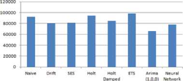
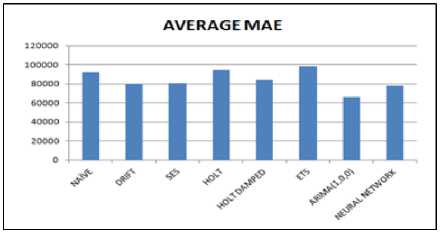
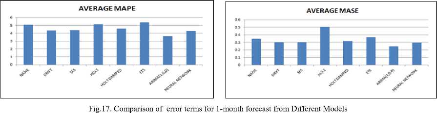
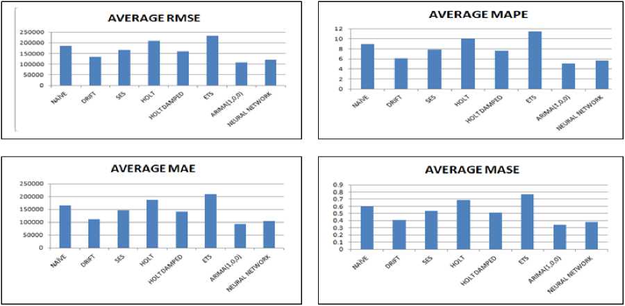
Fig.18. Comparison of error terms for 3-month forecast from Different Models

The result show forecasted values obtained data from different techniques used for prediction. The forecasted values obtained from Naïve, SES technique, Holt, ETS and neural network techniques have a significant difference as compared to actual test data set. For 1-month ahead forecast the average values of RMSE and MAE for Naïve, Drift, SES, Holt, Holt Damped, ETS, ARIMA and neural network are 92298, 79893.42, 81046.02, 94482.26, 84463.35, 98208.45, 65898.34 and 77788.43 respectively. The average value of error MAPE for Naïve, Drift, SES, Holt, Holt Damped, ETS, ARIMA and neural network is 5.06 %, 4.35%, 4.39%, 5.41%, 4.58%, 5.38%, 3.61% and 4.26% respectively. The another error component MASE for Naïve, Drift, SES, Holt, Holt Damped, ETS, ARIMA and neural network are 0.346744, 0.301997, 0.303965, 0.506124, 0.316636, 0.367113, 0.246216 and 0.294938 respectively. It is evident that value of all the error components RMSE, MAE, MAPE and MASE is less for ARIMA (1,0,0) in comparison to other forecasting techniques. Similarly for 3-month ahead forecast the value of all the error components are less for ARIMA (1,0,0) forecast as can be seen from table no-8 and figure 18. The significance of low error values is that forecasting results obtained from ARIMA (1,0,0) are closer to the test data set as compared to other forecasting techniques.

• V. Conclusion

This paper begins with an introduction of the importance of forecasting in relation to consumption of natural gas in industry. The foremost aim was to evaluate and compare the seven univariate forecasting techniques for forecasting the consumption of natural gas in industry. Due to limited data availability, forecasting horizon of one month and three month ahead forecast is selected. The out-of-sample forecasts are calculated by applying various forecasting techniques. Error components RMSE, MAE, MAPE, and MASE are used to compare the forecasted values of different forecasting techniques. It has evaluated from the comparison that all the error components are less for ARIMA(1,0,0) technique and the forecasted values obtained are closer to the actual consumption of natural gas.

Acknowledgment

The corresponding author is grateful to organization CFFP, BHEL, Haridwar for sharing their valuable contents with us.