Comparative study of inspired algorithms for trajectory-following control in mobile robot

Over the last few years, the interest in the machine learning and how it has been employed to help mobile robots in the navigation has been increased. Mobile robots have a lot of potential in the industry and in the house servant applications. Navigation control of wheeled mobile robots has been studied by many sources in the last decade ever after they are progressively used in an extensive range of applications. The motion of mobile robots must be modeled by mathematical calculation to estimate physical environment and run in delineated trajectories. At first, the research work was focused only on the kinematic model if there is optimum linear and angular velocity following [1]. Mobile robots are mostly used in manufacturing, healthcare and medicine [2].

The basic estimation problems in wheeled mobile robot trajectory-following are still waiting to be addressed; then the implicit essence of the motivation for this paper is to generate optimum control parameters for the mobile robot, to follow the required path with small trajectoryfollowing error, to beat unmolded kinematic disturbances, and to maintain the battery energy of the robot system. Traditionally, the problems of wheeled mobile robot controller have been processes by stabilizing point or by predetermined suitable problems like a trajectoryfollowing controller [3].

The navigation problem is the basic aim of a wheeled mobile robot in order that it requires a decision where to direct and that information is taken by an actual path. The problem of following may be classified into dynamic and kinematic trajectory-following control model. Kinematics controller targets are to reach angular and linear velocity as output to converge trajectory-following error to zero [4].

The modern survey of improvement nonholonomic control systems is illustrated in [5]. To the authors’ knowledge, the trajectory-following control problem is one of research challenges for robot nonholonomic mobile systems in but has yet to be widely studied. From past researches, an approximation for trajectoryfollowing control, back-stepping control has been applied to the trajectory-following control of robots [6] and is lately receiving expansive interest of researches about nonholonomic control systems.

Jiang and Pomet [7],utilized back-stepping theory for robot nonholonomic mobile systems by adaptation. Guldner and Utkin [8], suggested a Lyapunov theory to define a set of given configuration for required trajectories, then given a trajectory-following feedback controller to minimizing error and reducing chattering.

In this work, we propose an optimum back-stepping controller for solving trajectory-following problems for a robot nonholonomic mobile system, then a required trajectory with asymptotic stability can be obtained using the suggested control.

In engineering problems, the optimization is to detect a solution that can minimize or maximize a cost function. These days, the stochastic method is more often used to solve the optimization problem [9]. Recently, the nature-inspired algorithm is proving its ability in solving numerical problems of optimization more suitably. These optimization ways are improved to solve complex problems, such as scheduling of flow shop [10], highdimensional function optimization, reliability, and other engineering matters. Recently, many other algorithms have been used, like Artificial Bee Colony (ABC), Ant Colony Optimization (ACO), Particle Swarm Optimization (PSO), Harmony Search (HS) and Firefly Algorithm (FA).

Firefly Algorithm (FA) is a relatively new heuristic optimization algorithm, and it was first developed by Xin-She Yang. 2001 [11], which is based on the lighting of fireflies. Since then, it has been used to solve different problems of optimization, including function optimization, water apportionment network, groundwater modeling, structural design, energy-salvage, and others.

The remainder of this paper is organized as follows: Section 2 gives a Modeling of Differentiation Nonholonomic NI-Robot. Section 3 describes the Trajectory-Following Controller. Section 4 presents the Simulation. Conclusion is given in the final section.

• II.    Modeling Of Differentiation Nonholonomic NI- Robot

In this research, we consider a differentiation twowheeled drive mobile robot is collected of two standard drive wheels on the same axis and a free driving castor wheel for stability. In order that robot positioning, trajectory-following, the linear velocity, angular velocity and kinematic model, as shown in Fig. 1. The variables for this mathematical kinematic model of a differentiation two-wheeled drive mobile robot are an actual positional and angle parameterization (x , у , 6), desired positional and angle parameterization (x_T , у_т , 6_r), radius of each wheel (R_n) , centre of robot is (c) and length between two wheels ( L 1 ), together with linear and angular velocities (V, П), respectively [12].

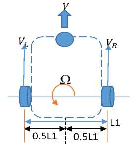
Fig.1. Model of a differentiation mobile robot.

At each instant in time, the left and right wheels follow a trajectory as shown in Fig. 2 that moves around the instantaneous centre of curvature mobile robot (ICCM) with the same angular rate [13].

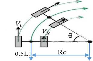
Fig.2. The instantaneous centre of curvature.

П(т) = d0(T)/dr

Thus:

V(t) = fi(T)Rc(T)

Vl(t) = (rc(t)+ ^1)п(т)

Vr(t) = (Rc(t) - у) П(т)

After solving Eqs. (3, 4) , we found the instantaneous centre of curvature mobile robot (ICCM) path close to the centre point axis (c) is given as Eq. (5) [13].

Rc(t) =

L i (V l (t)+V r (t))

2 (vL(t)-VR(t))

The angular velocity of the mobile robot is [14]:

П(т) = (vL(t)-VR(t))

'           Li

And the linear velocity of the mobile robot is [14]:

V(t) =

(V l (t)+V r (t))

Therefore, the prediction kinematic model shown in Eq. (8) . The constraint is non-holonomic, shown in Eq. (9) should be respected at rolling no spilling [15].

"xi  rcos(O)

^y = sin(0) - 0 И   0

01 [V]

1-1

— X(т)sin9(т) + у (т) COS9 (т) = 0

The (x, y, θ) parameterization can be explicit as

х(т) = x00 + j0тV(т)cos9(т)dт

У(т) = Уоо + JoтУ(т)sin0(т)dт

9(т)-91Ю + ^(т)(1т(12)

sliding mode kinematic controller to minimize the trajectory-following error, generates the perfect velocity control actions (linear and angular velocity) and tracks the desired trajectory-following coordinates.

The structure of trajectory-following control includes two parts; the first part is a nonlinear feedback acceleration control equation based on back-stepping control that controls the mobile robot to follow the predetermined suitable path; the second part is an optimization algorithm, that is performed depending on the Crossoved Firefly algorithm to tune the parameters of the controller to obtain the optimum trajectory-following variables.

The discrete kinematic model by using Euler’s theory with the instant time (L) and the sampling time (τ), can be expressed by Eqs. (13, 14, 15) :

x(L) = 0.5[V_r(L) + V_L(L)]cos9(L)kt + x(L — 1) (13)

y(L) = 0.5[V_r(L) + V_L(L)]sin9(L)bt + y(L — 1) (14)

9(L) = ^[V_r(L)+ V L (L)]^t+ 9(L— 1)    (15)

^R C

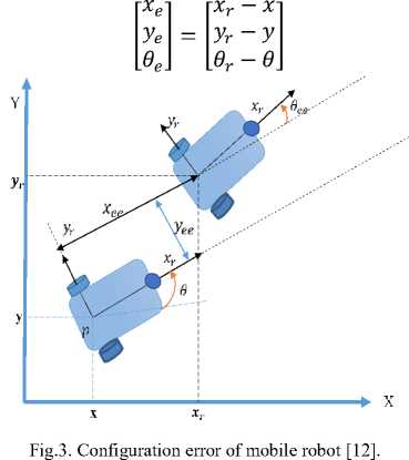
Finally, Fig. 3 show the configuration trajectoryfollowing error S_ee = [x_ee,y_ee,9_ee]^T can be presented by S ee = R* 6 ,where 6 = [x_e,y_e,9_e]^T and (R) rotational matrix, which can be shown by the Eqs. (16 ,17) [16]:

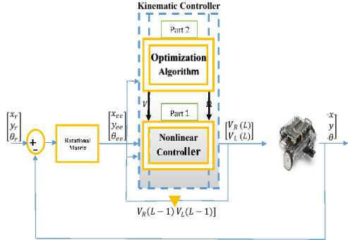
Fig.4. Structure of the nonlinear kinematic trajectory-following controller.

S

^S ee

Г ^x eel

=и

cos(9(т))   sin(9(т))  01 rxei

— sin(9(т))  cos(9(т))  0  l^yel    ⁽¹⁶⁾

0                 0         1J *-9e-*

• III.    Trajectory-Following Controller

• 3.1    Back-stepping Kinematic Controller

  Back-stepping is a method for nonlinear state feedback design by successive extensions of a Lyapunov function in order to guarantee stability. Two-step design procedure is known as back-stepping. Since a system starts at one desired output, and back-steps through the system selecting desirable values of the state components until the actual control input is reached. Since the integrator back-stepping procedure discovered by D.E. Koditscheck (1987) [17] for the first time. It has been applied to resolve the path tracking probleThe nonlinear trajectorytracking controller, which represented by the nonlinear feedback acceleration control approaches based on back-stepping execution and Lyapunov theory. The mobile robot nonholonomic kinematic model are transformed from cartesian actual parameterization to polar desired parameterization using that suggested control [18]. The suggested rule of controller that is responsible for finding the smooth and suitable actual right and left wheels velocity control action for nonholonomic mobile robot; thus, the trajectory-following error will be close to zero, and an asymptotically stable of system can be satisfied [19] , proposed nonholonomic control rule is illustrated in Fig. 5.

The proposed kinematic nonlinear controller is represented by the block diagram illustrated in Fig. 4. The Crossoved firefly algorithm optimization algorithm which is used to optimum tuning parameters of adaptive

The following two subsections are dedicated to explaining the nonlinear back-stepping kinematic controller and the proposed optimization algorithm to achieve tuning parameters of controls.

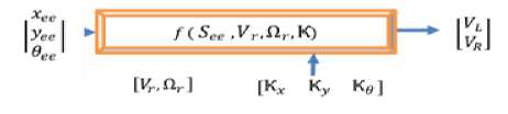
Fig.5. The kinematic nonlinear back-stepping structure.

HV : i=

Г V r cos(0_ee) + К х Х ее + L1/2(^ r + К у ^ У ее + К_е^ sin(0_ee) [V r COS⁽6_ee) + К^ — L1/2(ti_r + К у ^ y_ee + К_е^ sin⁽0_ee) (25)

The trajectory-following configuration transformation error Eq. (16) was used to facilitate the stability analysis and trajectory-following error closed loop system development. The derived configuration trajectoryfollowing error with state frame is See = [Х _ее,У _ее,6 _ее] can be expressed as Eq. (18) by Derivative of Eq. (16) and rearranging with Eq. (8) .

Lyapunov theory is used to demonstrate the stability of the control rule in order to become asymptotically stable at feedback system because this theory is access to a successful and simple method to getting the kinematic nonholonomic stability; thus, the constructional Lyapunov functions theory is described by Eq. (26) [13] :

V = | (% ee ²+У ee ²)+_^¹(1 — COS(0 ee ))    (26)

=

° ее

^x ее У ее 6 ее

V_rcos(9_(i e )+Уee^-V V_r Sin(9_ee) — Х_ее^ П_г-П

The derivative time of Equation (27) to be:

The desired virtual parameterization of the mobile robot shown as Eqs. (26, 20 and 21) which is based on the desired parameterization of the mobile robot S_r = [x_r,y_r, 6_r]^Tin [21].

^{V Х} ее^Хее ^{+ y} ее^уее ⁺ _и ⁶ ее ^sin(6ee^{)    (27)}

^К у

Substituting Eq. (24) in Eq. (18) , the derivative state

vector error becomes as follows [18]:

Xr = Vrcos6r(19)

Уг = Vrsin6r(20)

6r = ^r(21)

The required linear velocity and the required angular velocity for the required trajectory are shown by Eqs. (29 and 23) , respectively [13].

Vr = V(Xr)2 + (Уг)2(22)

Уг^-ХтУг ^r     (Х г )² + (У т )²

The cartesian actual velocity control rule V = f (S_ee ,V_r,^_r,K) such that lim_£ ^ _ro(S_r — S) = 0 is asymptotically stable can be determine with V_r > 0 and ^_r >  0 , for all т. Where S_ee , V_r, ^_r and К are the tracking-following model error , the reference linear and angular velocity and control gain, respectively, which must be the parameters of control are К_Х, К_у, К_д > 0 , so the control law as follows:

_ Г V1 _ [      ^Vr ^cos(6ee^{) + К}х^Хее     1

^Г Lol [fi_r + К_У^ У_ее + К д ^ sin(0_ee)]   ^{(  )}

Finally, the suggested kinematic nonlinear trajectoryfollowing control rule based on back-stepping theory and velocity (right and left wheels velocity) as a control action can be expressed by Eq. (25) [18].

S

ее

x ее y ее .6 ее

(^ r + V r (К у y_ee + К д sin(0_ee)))y_ee

^К х ^х ее

— (^ r + Ц-(К у у_ее + К д sin(0_ee⁾))y_ee + V r Sin⁽в ee ) .          —(К у V r У_ee + К_eV r Sin(0_ee))

Then,

V   ((^ r ⁺ ^ г (^К у ^уее ^{+ К}д ^sin ( ⁶ee^)))yee  ^Кх^хее^)хее

⁺ (-(^ r ⁺ ^ Т ( ^Ку ^уее

+ К д Sin ⁽ 9 ee⁾ ))У ee + V r Sin ⁽ 9 ee⁾ )

У ее + ^ (—(К у V r У ее + К д ^- Sin ⁽ 0 ee⁾ )) Sin ⁽ 0 ee⁾

^У                                        (29)

V = ^К _хХ ее² - V r К ^ Sin²0 ee <0      (30)

Clearly, V > 0. If S_ee = 0, V = 0. If S_ee ^ 0 , V > 0 and V < 0.if S_ee = 0,V = 0.if S_ee * 0 , V <  0 .

Then, V represents the Lyapunov function that will make the closed loop system globally asymptotically stable with three weighting parameters of control (К у ,К у ,К д )>0.

• 3.2    Swarm-Based Optimization Algorithms

• 3.2.1    Firefly Algorithm

• 3.2.1.1    Attractiveness

3.2.1.2 Distance

The stochastic algorithm which uses multiple agents (solutions) to move through the search space in the process of solving an optimization problem is known as the optimization algorithm. Some of these effective stochastic techniques that mimic the behaviours of certain animals or insects (birds, ants, bees, flies and even germs) are called Nature-Inspired Algorithm used for auto-tuning controllers. Two of these techniques are discussed here:

The firefly algorithm (FA), based on the behavior of fireflies flying towards an illumination source and their interaction with bioluminescent signals, is one of the algorithms relationship to the group of swarm algorithms (developed by Xin-She Yang [11]). The phenomenon of a firefly moving towards the brighter individual is the basis of the algorithm. One of the rules used in the firefly algorithm is that all fireflies are unisex. Furthermore, attractiveness of fireflies is proportional to the intensity of their sent-out light, where in the light intensity specified by the value of the objective function decreases with increasing distance between the fireflies. If there is no more attractive individual, a firefly moves randomly [20, 21].

Each firefly has a certain light intensity I, which varies according to the distance r between two individuals, and attractiveness A, which is proportional to the light intensity seen by the neighboring fireflies. Therefore, attractiveness (A) is dependent on distance and the light absorption coefficient у [21]:

A = A0e-yr2 (31)

where A0 denotes the attractiveness at r = 0.

The distance between any two fireflies m and n at X_m and X_n, respectively, is the Cartesian distance as follows:

^rmn =

llXm

—

X n l =

^^ L=1^(Xm,L

^Xn,L )

Where X_m , _L is the Lth component of the spatial coordinate X_m of Mth firefly and d is the number of dimensions.

3.2.1.3 Movement

The movement, during which the firefly m being in the location Xm tries to get closer to the brighter individual n in the position Xn is determined by the following equation [21]:

^Xm = ^Xm + ^A0^{e yr}™4 ^Xm ^{— X}n^)a1 (rand ^— 0) (33)

where Xm is the current location of a firefly mi, the second term denotes attractiveness and the third term is due to random movement (rand is a random number generator uniformly distributed in the range [0, 1], and α1 e [0,1]).

• 3.2.2    Crossoved Firefly Algorithm

In standard firefly algorithm, if there no brighter one than a firefly, the fireflies will move randomly, and by using flat crossover algorithms, the updating mechanism at each iteration by the coefficient delta is a uniform distributed random variable within optional interval [0,1]. The flat crossover coefficient (alpha) is defined as follows:

Alpha = (delta) * (alphal£era£ion )      (34)

Where alpha changing at each iteration. And the Flat crossover operated based on the following equation:

Xm=(alpha) * Xn + (1 — alpha) * Xn (35)

The possibilities of crossover are using to select fireflies instead of selecting randomly, then the candidates for the best solution are increasing. On the other hand, FA became needs less time to search for the best solution and its performance significantly development with the increases the population size because of decreasing the randomness, the pseudocode at algorithm 1.

Algorithm 1. The summarization of the computation procedure of CF algorithm

Step 1: Initialize the pop of fireflies X_m.

Step 2: Evaluate the fitness function f (X_m).

Step 3: Set Flash absorption coefficient у, A₀, al.

Step 4: Light intensity I_mat X_m is calculated.

Step 5: While the halting criteria is not satisfied do

For m=1: S (for all S fireflies).

For n=1: S (for all S fireflies).

if (In > Im) Movement all firefly       m towards n( d-dimension) by Eq. (33) concording to the luminousness between m and n can be determined by Eq. (31).

else

Movement all fireflies by Eq. (35) .

End if.

Evaluate the new fireflies and update flash intensities.

End for n

End for m

Step 6: Order the fireflies and find the best.

Step 7: End.

• 3.2.3    Design of Kinematic Nonlinear Controller based on CF Algorithm

This work introduced a Crossoved firefly algorithm to find the optimum parameter of control. The searching procedure of the suggested algorithm is described as follows:

• 1.    Initial searching elements of each firefly are created randomly within the determined range. Note that the

• 2.    The fitness function for each firefly can be calculated by the mean square error theory as Eq. (36) from [18]:

• 3.    Set step 3 to step 7 of the CF algorithm pseudo code to get the perfect value of controller’s gain by minimizing trajectory-following error.

• 4.    If the epochs number reach at max, then exit, else, go to step 2.

dimension of search space consists of all the control parameters needed in the back-stepping nonlinear control as described in Fig. 4.

(MSE)= 1 X ;7 ^; ; (.MLF - x(L) P )² + (y_r(£) P - y(L)^p)² + (0_r(L) P 0(L) P )² (36)

• IV.    Simulation

The aim of the simulations is to examine the effectiveness and performance of the proposed back-stepping kinematic nonlinear control depending on original firefly algorithm and CF optimization algorithms to a differentiation two-wheeled drive mobile robot by programming using MATLAB environment.

The resulting of a differentiation two-wheeled drive mobile robot trajectory-following, obtained by the suggested kinematic nonlinear control is involving trajectory-following, tracking-following error, the linear velocity of right and left wheel, linear and angular velocity of the mobile robot and (MSE). The execution of work can be simulated by the following table of the setting parameter (Firefly elements is equal to 3, NI-robot length is equal to 0.36 m and NI-robot radius is equal to 0.05 m).

Case study : ( Lemniscates trajectory)

The desired trajectory-following lemniscates, can be expressed by the following Equations:

x_r(f) = 0.75 + 0.75 * sin(2nT/50)      (37)

у_г(т) = sin(4nT/50)           (38)

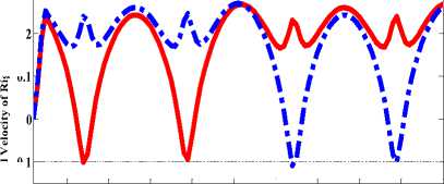
• •    The left and right velocity of back-stepping kinematic control based on original firefly algorithm is shown in Fig. 8, and for back-stepping kinematic controller based on CF learning is shown in Fig. 9.

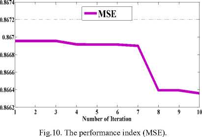
• •    The performance index MSE for parameterization trajectory-tracking during 10 epochs are described in Fig. 10 which is (0.866) for the proposed control based on original firefly learning algorithm and Fig. 11 which is (0.7957) for the proposed control based on CF in the simulation case study, which has perfect parameterization trajectory-following performance and it had the ability of generating suitable and smooth velocity without spike.

• •    Figure 12 proves the average of linear velocity (0.3 m/s) and the top peak of the angular velocity (±1 rad/s) of the NI robot for the proposed control based on original firefly learning algorithm and Fig. 13 proves the average of linear velocity (0.1m/s m/s) and the top peak of the angular velocity (±1rad/s) of the NI robot for proposed control based on CFA.

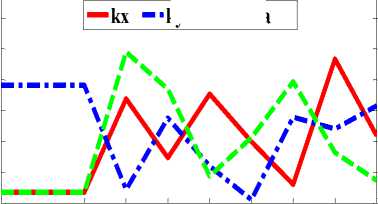
• •    Instantaneous suggested control parameters are shown in Fig. 14 which is tuned by using Crossoved firefly algorithm.

• •    The performance described in (Fig. 15, Fig. 16 and Fig. 17) for the proposed control based CF algorithm is obvious by showing the convergence of parameterization trajectory- following errors with small value.

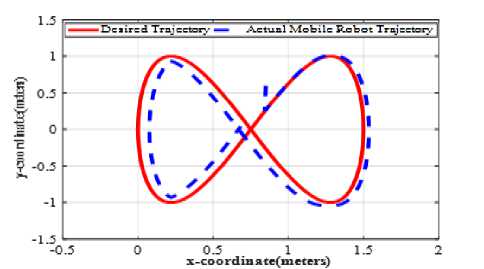
Fig.6. Actual and desired Lemniscates trajectory-following.

ДУ г (т)

0_г(т) = 2 tern ¹(

^(Ду.(г))² - (Ду г Ст))² +Д% г (т)

• •    The initial desired parameterization of robot at    q _r = [ 0.75,0,0 ] and the initial actual

parameterization of robot at q = [0,0,0], then the simulation of trajectory-following lemniscates of the NI mobile robot using back-stepping kinematic control based on original Firefly learning algorithm is viewed in Fig. 6. And the simulation of trajectory-following lemniscates of the NI mobile robot using back-stepping kinematic controller based on CF learning algorithm is viewed in Fig. 7.

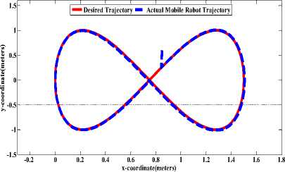
Fig.7. Actual and desired Lemniscates trajectory-following.

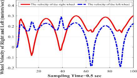
Fig.8. The right and left wheel velocity.

The velocity of the right wheel ■ The velocity of the left wheel

0.3

Е

0.2

0.1

10     20     30     40     50     60     70     80     90     100

Sampling Time=0.5 sec

-0.1

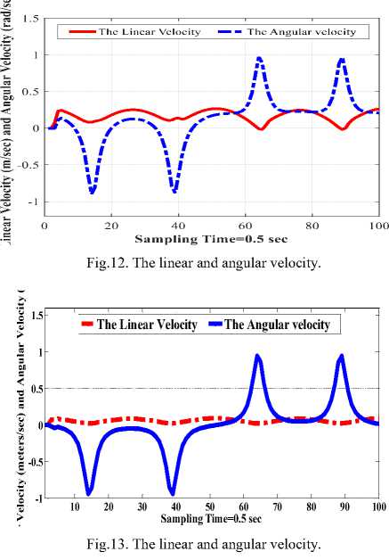
Fig.9. The right and left wheel velocity.

Performance Index (MSE)

ky ■ ■ ktheta

U

Е п

1        2       3       4       5        6        7        8        9       10

Sampling Time=0.5 sec

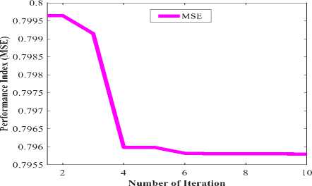
Fig.11. The performance index (MSE).

Fig.14. Control Parameters.

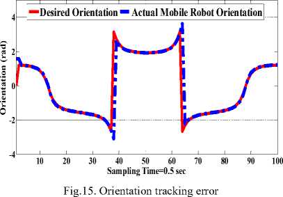
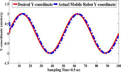
Fig.16. Position tracking error in Y- coordinate.

Alpha C

L

delta

A

A0

(кж,ку,ке)

L

L1

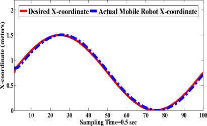
Fig.17. Position tracking error in X- coordinate.

R

a

Rc

r rand

R rmn

The trajectory-following nonlinear kinematic control based on back-stepping theory with two optimization algorithms for the differentiation nonholonomic two wheeled drive mobile robot have been presented in this work. The suggested controller examined by MATLAB (R2017b) set on National Instrument mobile robot (NI Mobile Robot). The simulation results show evidently the capability of robustness and adaptation of the suggested back-stepping kinematic controller based on Crossoved Firefly algorithm which optimum trajectory-following performance and it has the capability of generating more suitable and smooth velocities than the controller based on firefly algorithm because the CF algorithm has capability to get optimum controller parameters.

S

s ее

V

vd

V l

Vr (x,y,6)

(xr, yr, 6^)

^{( х}ее > У ее > ⁶ее" )

al

∆τ

List of Symbols

Ω ttd Ŗ τ

Ѵ Ѵ ̇

The flat crossover coefficient.

The mobile robot center (meter).

The dimensional vector of FA.

Parameter to reduce the randomness.

The flash intensity.

The intensity at the beginning.

The back-stepping control's gains

The number of samples for mobile robot

The length between each wheel and the robot axis of symmetry in y- guidance (m).

The radius of each wheel (rad). distance from the ICCM to the midpoint between the two wheels (c)

The distance between any two fireflies

The random number generator uniformly distributed in

[0, 1].

Real number

The Cartesian distance between fireflies.

The pose vector in the surface

The error vector

The linear velocity of the robot (meter/second).

The desired linear velocity of the robot (meter/second)

The linear speed of left mobile robot wheel (meter/second).

The linear speed of right mobile robot wheel (meter/second).

The        actual        pose

(position/orientation) of the robot.

The        desired       pose

(position/orientation) of the robot.

The configuration errors

The randomization parameter

The sampling period between two sampling times.

The angular velocity of the robot (rad/second).

The desired angular velocity of the robot (rad/second)

The rotation matrix

Real time.

Lyapunov functions

Time derivative of Lyapunov functions

Symbol       Definition

• [1]    Kumar D N, Samalla H, Rao Ch J, Naidu S, Jose K A, Kumar B M. Position and Orientation Control of a Mobile Robot Using Neural Networks[J]. Computational Intelligence in Data Mining, Smart Innovation, Systems and Technologies, 2015, 2(13): 123-131.

• [2]    Seo K, Lee J S. Kinematic path-following control of mobile robot under bounded angular velocity error[J]. Advanced Robotics, 2006, 20(1): 1-23.

• [3]    Kanayama Y, Kimura Y, Miyazaki F, Noguchi T. A stable tracking control method for an autonomous mobile robot[J]. IEEE International Conference on Robotics and Automation, 1990: 384-389.

• [4]    Zain A A, Daobo W, Muhammad S, Wanyue J, Muhammad Sh. Trajectory Tracking of a Nonholonomic Wheeleed Mobile Robot Using Hybrid Controller[J]. International Journal of Modeling and Optimization, 2016, 6(3): 136-141.

• [5]    Kolmanovsky I, McClamroch N H. Developments in nonholonomic control problems[J]. IEEE control systems, 1995: 20-26.

• [6]    Blazic S. A novel trajectory-tracking control law for wheeled mobile robots[J]. Robot. Auton. Syst. 59, 2011: 1001–1007.

• [7]    Jiang Z P, Pomet J B. Combining backstepping and timevarying techniques for a new set of adaptive controllers[J]. IEEE Int. Conf. Decision Contr.,1994: 2207–2212.

• [8]    Guldner J, Utkin V I. Stabilization of nonholonomic mobile robots using Lyapunov functions for navigation and sliding mode control[J]. IEEE Int. Conf. Decision Contr., 1994: 2967–2972.

• [9]    Geem Z W, Kim H J, Loganathan G V. A new heuristic optimization algorithm: Harmony search[J]. SAGE Journals, ,2001, 76(2): 60-68.

• [10]    Adithyan T, Vasudha Sh, Gururaj B, Chandrasegar Th. Nature inspired algorithm[C]. International Conference on Trends in Electronics and Informatics (ICEI), pp. 1131 – 1134.

• [11]    Yang X S. Firefly Algorithms for Multimodal Optimization[J]. SAGE Journals, vol. 5792, pp. 169– 178,2009.

• [12]    Nizar H, Basma J. Trajectory Tracking Controllers for Mobile Robot: Modeling, Design and Optimization[M]. Lambert Academic Publishing, 2016.

• [13]    Al-Araji A. Design of a cognitive neural predictive controller for mobile robot[M]. Ph.D. thesis, Brunel University, United Kingdom, 2012.

• [14]    Nizar H, Basma J. Design of a Kinematic Neural Controller for Mobile Robots based on Enhanced Hybrid Firefly-Artificial Bee Colony Algorithm[J]. AL -Khwarizmi Engineering Journal, vol. 12, no. 1, pp. 4560 ,2016.

• [15]    Ye J. Adaptive control of nonlinear PID-based analogue neural network for a nonholonomic mobile robot[J]. Neurocomputing, vol. 71, no. 7, pp. 1561-1565 , 2008.

• [16]    Yousif Z, Hedley J, Bicker R. Design of an adaptive neural kinematic controller for a national instrument mobile robot system[J]. IEEE International Conference on Control System, Computing and Engineering, pp. 623628, 2012.

• [17]    Yuan G. Tracking Control of a Mobile Robot using Neural Dynamics based Approaches[M]. Master Thesis, University of Guelph, 2001.

• [18]    Al-Araji A. Development of kinematic path-tracking controller design for real mobile robot via back-stepping slice genetic robust algorithm technique[J]. Arab J. Sci. Eng. vol. 39, no. 4, pp. 8825–8835, 2014.

• [19]    Al-Araji A. Design of on-line nonlinear kinematic

  trajectory tracking controller for mobile robot based on Optimal Back-Stepping Technique[J]. Iraqi Journal of Computers, Communications, Control and Systems Engineering. vol. 2, no. 14, pp. 25-36, 2014.

• [20]    Xing B, Gao W J. Innovative Computational Intelligence: A Rough Guide to 134 Clever Algorithms[J]. Computational Intelligence and Complexity, 2014.

• [21]    Yang X S. Nature-Inspired Metaheuristic Algorithms[M]. Second Edition, Luniver Press, 2010.