Comparison of Four Interval ARIMA-base Time Series Methods for Exchange Rate Forecasting

Published Online July 2015 in MECS DOI: 10.5815/ijmsc.2015.01.03

generating process or when there is no satisfactory explanatory model that relates the prediction variable to other explanatory variables.

Exchange rate is one of the most effective variables in financial environments and forecasting of it is very important for economic decision makers and financial managers. In exchange rate field, numerous forecasting investigations have been accomplished [2-5] that number of these investigations represent the mentioned issue importance. Nowadays, despite of obtainable numerous financial forecasting models, accurate forecasts of exchange rate are not easy task. It is the main reason that researches for obtaining more accurate results have not been stopped [6-11].

Time series forecasting is an important area of forecasting in which past observations of the same variable are collected and analyzed to develop a model describing the underlying relationship. The model is then used to extrapolate the time series into the future. This modelling approach is particularly useful when little knowledge is available on the underlying data generating process or when there is no satisfactory explanatory model that relates the prediction variable to other explanatory variables [12].

Several models have been suggested for time series forecasting, that are generally divided to linear and nonlinear models. One of the most important and widely used linear time series models is the Auto-Regressive Integrated Moving Average ( ARIMA ) model that has enjoyed fruitful applications in forecasting social, economic, engineering, foreign exchange, and stock problems. Second class of time series forecasting is nonlinear time series models. Artificial neural networks are one of these models that are able to approximate various nonlinearities in the data and are flexible computing frameworks for modelling a broad range of nonlinear problems [13].

One significant advantage of the ANN models over other classes of nonlinear model is that ANNs are universal approximators, which can approximate a large class of functions with a high degree of accuracy. No prior assumption of the model form is required in the model building process. Instead, the network model is largely determined by the characteristics of the data. Commonly used network models include multi-layer perceptron ( MLP ), Radial Basis Function ( RBF ), Probabilistic Neural Networks ( PNN s) and General Regression Neural Networks ( GRNNs ) [14]. Single hidden layer feed-forward network is the most widely used model form for time series modelling and forecasting [15].

Forecasting accuracy is one of the most important factors to choose the forecasting method, and regardless numerous time series forecasting models, the accuracy of time series forecasting is fundamental to many decision processes and hence the research for improving and diagnosing the effectiveness of forecasting models has been never stopped. Ture has compared the performance of four different time series models to forecast the hepatitis A virus infection [16]. Taylor et al have compared the univariate methods for forecasting electricity demand [17]. Kima [18] has forecasted the international tourist flows to Australia for comparison between the direct and indirect methods. Cho also has compared the three different approaches to tourist arrival forecasting [19]. Some other research in this field, consist of Weatherforda [20] to hotel revenue management forecasting, Smith [21] to traffic flow forecasting and Sfetsos [22] to mean hourly wind speed time series forecasting.

In the financial field also is accomplished various research similar above. Alon has compared the performance of artificial neural networks and traditional methods to aggregate retail sales forecasting [23]. Meade [24] has compared the accuracy of short-term foreign exchange forecasting methods. Leunga et al [25] have compared the classification and level estimation models to forecasting the stock indices. Lisi also has compared the neural networks and chaotic models for exchange rate prediction [26]. Tsui [27] has compared the exchange rate and pricing behaviour between Taiwan and Japan for manufacturing industries. Ghosh [28] has compared the effects of exchange rate regime choice in emerging markets with advanced and low-income nations for 1999–2011. Wang et al [29] have compared the characterizing information flows among spot, deliverable forward and non-deliverable forward exchange rate markets: A cross-country comparison. Razavi et al [30] have compared the circuit patency and exchange rates between two different continuous renal replacement therapy machines.

In this paper, is compared the performance of four different interval time series methods for financial markets forecasting. The rest of the paper is organized as follows. In the next section, concepts of four time- series methods: Auto-Regressive Integrated Moving Average (ARIMA), Fuzzy Auto-Regressive Integrated Moving Average (FARIMA), Fuzzy Artificial neural Network (FANN) and Hybrid Fuzzy Auto-Regressive Integrated Moving Average (FARIMAH) are reviewed. Empirical result from forecasting the exchange rate (US Dollar/Rial) is reported in Section 3. The performance of each model is compared in section 4, and finally the conclusions are discussed.

• 2.    Time Series Forecasting Models

• 2.1.    The Auto-Regressive Integrated Moving Average (ARIMA) model

• 2.2.    The Fuzzy Auto-Regressive Integrated Moving Average (FARIMA) model

There are several different approaches to time series modeling. Interval models are special class of quantitative forecasting models. These models calculate an interval as optimum forecast of independent variable. In this section are reviewed four different interval time series models.

In an autoregressive integrated moving average model, the future value of a variable is assumed to be a linear function of several past observations and random errors. That is, the underlying process that generate the time series has the form yt =θ0+ϕ1yt-1+...+ϕpyt-p+εt-θ1εt-1-...-θqεt-q                                        (1)

where y _t and ε _t are the actual value and random error at time period t , respectively; φ _i ( i = 1,2,..., p ) and θ _j ( j = 1,2,..., q ) are model parameters. p and q are integers and often referred to as orders of the model. Random errors, ε _t , are assumed to be independently and identically distributed with a mean of zero and a constant variance of σ ² .

The Box–Jenkins [31] methodology includes three iterative steps of model identification, parameter estimation and diagnostic checking. The basic idea of model identification is that if a time series is generated from an ARIMA process, it should have some theoretical autocorrelation properties. By matching the empirical autocorrelation patterns with the theoretical ones, it is often possible to identify one or several potential models for the given time series. Box and Jenkins [31] proposed to use the autocorrelation function ( ACF ) and the partial autocorrelation function ( PACF ) of the sample data as the basic tools to identify the order of the ARIMA model.

Once a tentative model is specified, estimation of the model parameters is straightforward. The parameters are estimated such that an overall measure of errors is minimized. This can be done with a nonlinear optimization procedure. The last step of model building is the diagnostic checking of model adequacy. This is basically to check if the model assumptions about the errors, ε _t , are satisfied.

Several diagnostic statistics and plots of the residuals can be used to examine the goodness of fit of the tentatively entertained model to the historical data. If the model is not adequate, a new tentative model should be identified, which is again followed by the steps of parameter estimation and model verification. Diagnostic information may help suggest alternative model(s). This three-step model building process is typically repeated several times until a satisfactory model is finally selected. The final selected model can then be used for prediction purposes [32].

The parameter of ARIMA(p, d, q), ϕ ,ϕ ,....ϕ,   and θ ,θ ,....θ,  are crisp. Instead of using crisp, fuzzy parameters, ϕ~1,ϕ~2,....ϕ,~p and θ~1,θ~2,....θ,~q , in the form of triangular fuzzy numbers are used in Fuzzy Auto-

Regressive Integrated Moving Average models [33]. A fuzzy ARIMA (p, d, q) model is described by a fuzzy function with a fuzzy parameter:

ф p ( в ) w = ~_q ( в a.

W=(1- B)d (Zt - ц)(3)

W = (W-1 + (Wt-2 +.... + (pWt-p + a. -~p+1 a.-1 -~p+2a.-2 -...-~p+qa.-q(4)

~~~ where {Zt} are observations, (,(2,....(p and 91,02,....0q, are fuzzy numbers. Eq. (4) is modified as

~~   ~      ~      ~    ~~

W t = P W . - J + P f W t - 2 + .... + P p^W. - p ⁺ a . ^- P p + 1 a . - 1 ^- P p + 2 a t - 2 ^- ... ^- P p + q a t - q

Fuzzy parameters in the form of triangular fuzzy numbers are used:

цP^Pi )=?

I «I- Pi\ c _i

P  ai-ci ^Pi^ai+ ci, otherwise,

where ц ~ ( p, ) is the membership function of the fuzzy set that represents parameter p i , a i is the center of the fuzzy number, and c i is the width or spread around the center of the fuzzy number. Using fuzzy parameters p i in the form of triangular fuzzy numbers and applying the extension principle, it becomes clear [34] that the membership of W in Eq. (5) is given as

Ц w ( W . ) = ] ¹

W t - I p^.-i- a . + 2 p^a. + p - i Z i = 1 c i W t - i | + 2 p ++ 1 c i\ a . + p - i|

for  W_t * 0,    a . * 0

otherwise

Simultaneously, Z _t represents the t th observation, and h -level is the threshold value representing the degree to which the model should be satisfied by all the data points y , y , , y to a certain h -level. A choice of the h - level value influences the widths c of the fuzzy parameters:

Ц у ( y . ) > h       fort = 1,2,...k

The index t refers to the number of nonfuzzy data used for constructing the model. On the other hand, the fuzziness S included in the model is defined by p k               p+q k

S=EE 4 f^+ZE 4 Pi-pa+p-il i =1 t =1                  i=p+1 t =1

where p_ is the autocorrelation coefficient of time lag i-p, f is the partial autocorrelation coefficient of time lag i . The weight of c _i depends on the relation of time lag i and the present observation, where the p of AR (p) is derived by PACF and the q of MA (q) is derived by ACF . Next, the problem of finding the fuzzy ARIMA parameters was formulated as a linear programming problem:

p k                 p + q k

Minimize

S=EE CifiiWt -il+EE cP - pkt+p - il i=1 t=1                     i=p+1 t=1

p

E aiWt - i + at i=1

p + q

- E aiat+p - i i=p+1

+

( i + h ) e c i W t - i i + E c i a

( p

p + q          )

t + p - i

^ i + 1                i = p + 1              у

<1 г w

t = 1,2,.., k

p

E “Wt - i + at i=1

p + q

- E «-at+p-i i=p+1

( p

p + q          )

+

( 1 + h ) E c i W t - i l+ E c i a

t + p - i

₄ i + 1                i = p + 1              у

, | s W t

t = 1,2,.., k

c i >  0 fori = 1,2,..., p + q

At last, according to the Ishibuchi and Tanaka [35] opinion, the data around the model's upper bound and lower bound is deleted when the fuzzy ARIMA model has outliers with wide spread, and then reformulating the fuzzy regression model.

• 2.3.    The Fuzzy Auto-Regressive Integrated Moving Average (FARIMA) model

The Forecasted interval of Fuzzy Auto-Regressive Integrated Moving Average models is extended in some specific data conditions [36]. According to the Ishibuchi and Tanaka opinion, forecasting interval can be too wide, when training data set includes the significant difference or outlying case [35]. In improved model, the diagnosis ability of Probabilistic Neural Networks (PNNs) [37] is used in order to recognize the more probably spaces in forecasted interval of FARIMA model. Technically, PNN is a classifier and is able to deduce the class/group of a given input vector after the training process is completed. PNN is conceptually built on the Bayesian method of classification which, given enough data, is capable of classifying a sample with the maximum probability of success [38]. The procedure of improved model is as follows:

Phase I: Fitting the FARIMA model using the available information of observations. The result of phase I is as follows:

~

W_t = a « 1 , cn W_t - 1 + ■■■ + a ^a p , c p w - p + a t ^- a p p + 1 , c p + 1 / a t - 1 ^- ■■■■ ^- a p + q , c p + q / a t - q ,

where W_t = ( 1 - B ) d ( Z _t - ц ) , a i is the center of the fuzzy number, and c i is the width or spread around the center of the fuzzy number. Obtained interval of FARIMA model is divided to n equal sections to use in probabilistic neural network. The subinterval which includes the real value or n-1 other subintervals is considered as target data to neural network. Other information, include result of FARIMA and time series data is considered as train data.

Phase II: Designing and training one network to recognize the more probably spaces in forecasted interval of FARIMA model. The result of this phase is one interval with 1/n width and a confidence coefficient ( a is the diagnosis ability of PNN in test data). In improved model, it is assumed that desired case only is one of the n divided subintervals, but generality, the each k consecutive or nonconsecutive subinterval of n divided subinterval can be selected as desired case.

• 2.4.    The Fuzzy Artificial Neural Network (FANN) model

A hybrid model is described by a fuzzy function with a fuzzy parameter: qp

~ = f ⁽ b о + ^ w j ■ g ⁽ b о j + ^ ^wi , j ■ y_t - i ))

j=1                 i =1

~~ where yt are observations, w~j , w~i, j , b0,b0, j are fuzzy numbers. Eq. (12) is modified as qq

~~~

~t = ^{f (} b о + ^ ^wj ■ Xt , j ) = ^f ( ^ ^wj ■ Xt , j )

j=1

p where   Xt,j = g(b0j + ^ wi,j ■ yt-i)   . Fuzzy i=1

numbers w i , j = ( ti i , j , b , j , c i , j ) are used:

parameters in the form of triangular fuzzy

	bi,j	w - » i,J	- ai,j )
^ w , ,( wi j=-	bi,j	( wtj - c i,j	- ci,j )

if     Oi,j < WiJ < bi, j, if     bi,j < wu < ci,j,

otherwise,

where ^ w ( w i j ) is the membership function of the fuzzy set that represents parameter w i j . Applying the

~ extension principle [39], it becomes clear that the membership of X

p

=g(^ wi,j ■ yt-i)in Eq.(13) is given i=0

as follows:

^A x)

( x ,j ^- g ( S p = oa.j • y. - i ) )

g ( S p = .b • у - )^- g ( S p = o a .j ■ y. - i )

¹f  g ( S ^p = o a -.j • y . - - ) <  x.j <  g ( S poKj • y . - i )-

( x.j ^- g ( S p = oc.j • y . - . ) )

g ( S p = ob.j • у - . )^- g ( S ^p = o c .j • у - . )

¹f  g ( S ^p = o b -.j • y . - . ) ^ x ..j ^ g ( S ^p = oc-j • y . - . ) -

l o

otherwise

With consider triangular fuzzy numbers X ^~ _{t , j} with membership function as Eq. (15) and triangular fuzzy parameters w _j as follow

HWjVwJ )=<

eJ -

— (wj - dj ) dj

if

d j <  w j <  e j .

^eJ ^{- f}j

if

e j ^ w j ^ f j .

otherwise,

The membership function of ^~ y

—

= f (b o +

q

S Wj j=1

q

• X~.,j) = f (S wj • X~.,j) is given as j=0

- B 1 + 2 A ₁

My(y, )S]

B^- + 2 A ₂

Where

B1- 1

2 A1 J

B2_ 1 2 A ₂ J

—

—

C 1 - f "1 ( y . )

A 1

2

C 2 - f "1 ( y . )

A ₂

2

otherwise ,

if

if

C i <  f "¹ ( y . ) < C з ,

C 3 <  f -¹ ( y . ) < C 2 ,

n vq ( j ГJ C —        d, • g       a • y

• ¹   2— i j = 0 1 ^j °( Z—n = o   ¹,^{j J} t ¹ J J

• 3.    Application of Hybrid Model to Exchange Rate Forecasting

  In order to demonstrate the more appropriateness and more effectiveness model of the four reviewed models, consider the following application of forecasting the exchange rate (US Dollar/Iran Rial). The information of this investigation consists of 42 daily observations from 5 Nov to 16 Des 2005 (Ref: Centre Bank of Iran (CBI)), Fig. 1.

q (      (p           ))

C2 =LJ=o(fj • g(L—oci,j ' y1 -JJ’ q (   (V p

^C з = L j = o ( e j'^g ( L = o ^b-j y t -JJ ’

Now with consider threshold level h for all membership function value of observations according to Eq. (8) the nonlinear programming is given as follow [40]:

Min	lL l q t = 1 - B 1 2 А Г +	( /■     (V^ P =o 1 f j • g ( L . =		0 c i , j - f - A 1	• y t - i y ,)	J-( d j • g ( L =o ° - , j • y t - - JJ
		"( jl ( 2 A i	J- C^			1 /2 < h	if	C 1 <  f - 1 ( y t ) < C 3 , for	t —1,2,.... k
Subject . to
	-B 2-+ 2 A 2	"( B^ _l 2 A 2	J- C 2	- f - A	( y t )	1 /2 < h	if	C з <  f - 1 ( у , ) < C„ for	t — 1,2,.... k

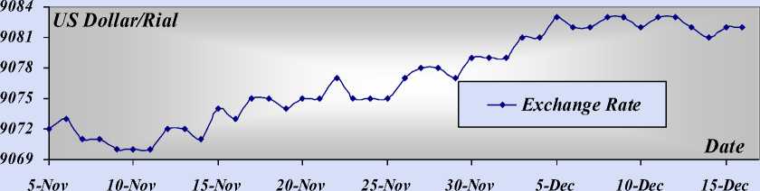
Fig. 1. Exchange Rate data from 5 Nov to 16 Des 2005 . Ref: Centre Bank of Iran ( CBI ).

• 3.1.    The forecasts

• 3.1.1.    The Auto-Regressive Integrated Moving Average (ARIMA) model

• 3.1.2.    The Fuzzy Auto-Regressive Integrated Moving Average (FARIMA) model

  Using Setting ( a , a , a ) = ( 9060.05,0.607,0.421 ) , the fuzzy parameters obtained using Eq. (10) (with h=0) are shown in Eq. (20).

In all models, is used the first 35 observations to formulate the model and the next 7 observations to evaluate the performance of the model.

Using the Eviews package software, the best-fitted model is ARIMA (2, 1, 0) as follows. The actual value and 95% of the confidence interval of ARIMA model are given in Table. 1.

Z_t = 9060.5 + 0.607Z_t_, + 0.421Z_t_ ₂ + a_t.

Table 1. Actual value and 95% of the confidence interval of ARIMA model.

Date	Actual value	Lower bound	Upper bound	Date	Actual value	Lower bound	Upper bound
10- Des	9082	9074	9090	14- Des	9081	9073	9089
11- Des 12- Des	9083 9083	9075 9075	9091 9091	15- Des	9082	9074	9090
13- Des	9082	9074	9090	16- Des	9082	9074	9090

Z = 9060.5 + ( 0.607,0.00028 Z, , + ( 0.421,0.0 Z_{t 2} + a_t.

It is known from the above results that the observation of 15 Nov is located at the upper bound (outlier), so the LP constrained equation that is produced by this observation is deleted and renews phase II, let h=0 then we get the model that is in Eq. (21). The results are plotted in Fig. 4 and shown in Table 2.

Z_t = 9060.5 + ( 0.607,0.00023 Z_t , + ( 0.421,0.0 Z_{t 2} + a_t.

Table 2. Actual value and forecasted interval of FARIMA model.

Date	Actual value	Lower bound	Upper bound	Date	Actual value	Lower bound	Upper bound
10- Des	9082	9081	9085	14- Des	9081	9080	9084
11- Des 12- Des	9083 9083	9080 9081	9084 9085	15- Des	9082	9079	9083
13- Des	9082	9081	9085	16- Des	9082	9080	9084

Using the obtained best-fitted model is ARIMA (2, 1, 0) as follow. The actual value and 95% of the confidence interval of ARIMA model are given in Table. 2.

• 3.1.3.    The Improved FARIMA with Probabilistic Neural Networks (FARIMAH) Model

In improved model after FARIMA model is used Probabilistic Neural Networks. The optimum network is a network with five input neuron and one output neuron. The structure of designed network is given in Fig. 2.

Probabilistic

Neural Network

Oiiipui Unit

Inpiu Variables

Fig. 2. The structure of designed network.

Where

Vari: forecasted lower bond of time series in time t ( L _t )

Var2: Forecasted upper bond of time series in time t ( U _t )

Var3: Forecasted value of time series in time t ( Z _t )

Var4: Difference between forecasted value of time series in time t & t-1 ( Z ^ˆ _t - Z ^ˆ _{t - 1} )

Var5: Difference between forecasted upper bond (lower bond) of time series in time t & t-1 ( U _t - U _{t - 1} )

Obtained result of upper and lower bound forecasting with improved model with 100% confidence coefficient is given in Table 3.

Table 3. Actual value and forecasted interval of PNN/FARIMA model.

Date	Actual value	Lower bound	Upper bound	Date	Actual value	Lower bound	Upper bound
10- Des	9082	9080	9083	14- Des	9081	9080	9083
11-    Des 12-    Des	9083 9083	9081 9080	9084 9083	15- Des	9082	9079	9082
13- Des	9082	9080	9083	16- Des	9082	9081	9084

• 3.1.4.    The Fuzzy Artificial Neural Network (FANN) model

With consider concepts artificial neural networks designing [41] and using MATLAB7 package software, the best fitted network is N^(3-3-1) . The mentioned network is shown in Fig. 3. The weights and biases of mentioned network also are given in Table 4.

Table 4. Weights and biases of final network.

Input Weights			Hidden Weights	Biases
W1 i,1	W1 i,2	W1 i,3		b1j	b2
-3.3947	1.9112	11.9393	3.3696	-2.7097	-4.0598
-2.3734	-0.31743	-28.5843	6.2053	2.3013
6.8024	-3.6088	-27.0192	-1.1491	28.9588

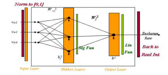
Fig. 3. Structure of the best fitted network, N(3-3-1).

Setting ( a * , a * , a ** ) = ( 9060.05,0.607,0.421 ) and ( a * , a * , a * , a * ) = ( 3.37,6.205, - 1.149, - 4.060 ) , the fuzzy parameters are obtained using Eq. (18) (with h=0) are shown in Eq. (22). Worthy of mention that in this case the triangular fuzzy numbers is considered symmetric, output neuron transfer function is considered linear and connection weight between hidden and input layer is considered crisp.

Z_t = 9060.5 + 00.607,0.00008}Z- + {0.421,00)} Z_t_₂ -44.66,0.088} X_t0

+ ( 3.37,0.0 X_{t> 7} + ( 6.205,0.0 X_t>2 - 010^9^)0)0)} X_t3.

Using the revised hybrid model, the future value of the gold price of the next 5 transaction days is forecasted, whose results are shown in Table 5.

Table 5. Actual value and forecasted interval of Hybrid model.

Date	Actual value	Lower bound	Upper bound	Date	Actual value	Lower bound	Upper bound
10- Des	9082	9081	9084	14- Des	9081	9081	9084
11- Des	9083	9082	9084
				15- Des	9082	9081	9084
12- Des	9083	9082	9084
13- Des	9082	9081	9084	16- Des	9082	9081	9084

• 4.    Comparison the Performance of Models

In this section, based on the empirical results of this example, the predictive capabilities of the models are compared together. The information of forecasted interval width and related performance of each model is given in Table 6.

Table 6. He information of forecasted interval width and related performance of each model.

Model	Forecasted interval width	Related Performance
		ARIMA	FARIMA	PNN/FARIMA	Fuzzy & ANNs
ARIMA	16.2	0	-	-	-
FARIMA	4.2	74.1%	0	-	-
PNN/FARI MA	3.1	80.9%	26.2%	0	-
Fuzzy & ANNs	2.5	84.6%	40.5%	19.4%	0

According to the above result between mentioned models in exchange rate forecasting, the Auto-Regressive Integrated Moving Average model has lowest performance and the hybrid artificial neural networks and fuzzy logic model has better performance than other models.

In today's world, using quantitative methods for forecasting the financial markets, improvement of decisions and investments is transformed to undeniable exigency. Nowadays, regardless numerous time series forecasting models, the accuracy of time series forecasting is fundamental to many decision processes and hence the research for improving and diagnosing the effectiveness of forecasting models has been never stopped. In this paper are compared the performance of four different interval time series methods (Auto-Regressive Integrated Moving Average (ARIMA), Fuzzy Auto-Regressive Integrated Moving Average (FARIMA), Hybrid ANNs and Fuzzy, Improved FARIMA) to exchange rate forecasting. Empirical results of exchange rate forecasting indicate that the hybrid ANNs and Fuzzy model is more satisfactory than other models.

The author would especially like to thank, Mr. Majid Rafiei who greatly helped me in collecting necessary data.

• [1]    M. Khashei, "Soft Intelligent Decision Making (SIDM)", Ph.D. Thesis, Isfahan University of Technology (IUT), Industrial Engineering Department, 2013.

• [2]    M. CaZorzi, A. Kocięcki, M. Rubaszek, “Bayesian forecasting of real exchange rates with a Dornbusch prior”, Economic Modelling, Vol. 46, Pages 53-60, 2015.

• [3]    T. Korol, “A fuzzy logic model for forecasting exchange rates” , Knowledge-Based Systems, Vol. 67, Pages 49-60, 2014.

• [4]    O. Ince, “Forecasting exchange rates out-of-sample with panel methods and real-time data” , Journal of International Money and Finance, Vol. 43, Pages 1-18, 2014.

• [5]    J.A. Batten, H. Kinateder, N. Wagner, “Multifractality and value-at-risk forecasting of exchange rates” , Physica A: Statistical Mechanics and its Applications, Vol. 401, Pages 71-81, 2014.

• [6]    A. Garratt, E. Mise, “Forecasting exchange rates using panel model and model averaging” , Economic Modelling, Vol. 37, Pages 32-40, 2014.

• [7]    M. Rout, B. Majhi, R. Majhi, G. Panda, “Forecasting of currency exchange rates using an adaptive ARMA model with differential evolution based training”, Journal of King Saud University - Computer and Information Sciences, Vol. 26, Issue 1, Pages 7-18, 2014.

• [8]    C. Pierdzioch, J. Rülke, “On the directional accuracy of forecasts of emerging market exchange rates” , International Review of Economics & Finance, Vol. 38, Pages 369-376, 2015.

• [9]    D. Ferraro, K. Rogoff, B. Rossi, “Can oil prices forecast exchange rates? An empirical analysis of the relationship between commodity prices and exchange rates” , Journal of International Money and Finance, Vol. 54, Pages 116-141, 2015.

• [10]    L. Morales-Arias, G. V. Moura, “Adaptive forecasting of exchange rates with panel data”, International Journal of Forecasting, Vol. 29, Issue 3, Pages 493-509, 2013.

• [11]    D. Zhou, “A New Hybrid Grey Neural Network Based on Grey Verhulst Model and BP Neural Network for Time Series Forecasting”, International Journal of Mathematical Sciences and Computing, Vol. 5, No. 10, Pages 114-120, 2013.

• [12]    Khashei, M., Bijari, M., “Hybridization of the probabilistic neural networks with feed–forward neural networks for forecasting”, Engineering Applications of Artificial Intelligence, Vol. 25, pp. 1277– 1288, 2012.

• [13]    M. Khashei, M. Bijari, “An artificial neural network (p, d, q) model for time series forecasting”, Expert Systems with Applications, vol. 37, pp. 479– 489, 2010.

• [14]    M. Khashei, "Using general regression neural networks (GRNN) for forecasting", Behbod Journal, Isfahan University of Technology, 133, (2006), 28.

• [15]    Zhang, P, Min Qi b, G, "Neural network forecasting for seasonal and trend time series", European Journal of Operational Research 160, 501–514, 2005.

• [16]    M. Ture, I. Kurt, "Comparison of four different time series methods to forecast hepatitis A virus infection", Expert Systems with Applications 31 (2006) 41–46.

• [17]    J. W. Taylor, L. M. de Meneze, P. E. Mc Sharry, "A comparison of univariate methods for forecasting electricity demand up to a day ahead", International Journal of Forecasting 22 (2006) 1– 16.

• [18]    J. H. Kima, I. A. Moosab, "Forecasting international tourist flows to Australia: a comparison between the direct and indirect methods", Tourism Management 26 (2005) 69–78.

• [19]    V. Cho, "A comparison of three different approaches to tourist arrival forecasting", Tourism Management 24 (2003) 323–330.

• [20]    L. R. Weatherforda, S. E. Kimesb, "A comparison of forecasting methods for hotel revenue management", International Journal of Forecasting 19 (2003) 401–415.

• [21]    B. L. Smith, B. M. Williams, R. Keith, "Comparison of parametric and nonparametric models for traffic flow forecasting", Transportation Research Part C 10 (2002) 303–321.

• [22]    A. Sfetsos, "A comparison of various forecasting techniques applied to mean hourly wind speed time series", Renewable Energy 21 (2000) 23-35.

• [23]    I. Alon, R. J. Sadowski, "Forecasting aggregate retail sales: a comparison of artificial neural networks and traditional methods", Journal of Retailing and Consumer Services 8 (2001) 147-156.

• [24]    N. Meade, "A comparison of the accuracy of short term foreign exchange forecasting methods", International Journal of Forecasting 18, (2002) 67–83.

• [25]    M. T. Leunga, H. Daoukb," Forecasting stock indices: a comparison of classification and level estimation models", International Journal of Forecasting 16 (2000) 173–190.

• [26]    F. Lisi, R. A. Schiavo, "A comparison between neural networks and chaotic models for exchange rate prediction", Computational Statistics & Data Analysis 30, (1999) 87-102.

• [27]    Hsiao-Chien Tsui, “Exchange rate and pricing behavior: Comparison of Taiwan with Japan for manufacturing industries”, Japan and the World Economy, Vol. 20, Pages 290-301, 2008.

• [28]    Amit Ghosh, “A comparison of exchange rate regime choice in emerging markets with advanced and low income nations for 1999–2011”, International Review of Economics & Finance, Vol. 33, Pages 358-370, 2014.

• [29]    Kai-Li Wang, Christopher Fawson, Mei-Ling Chen, An-Chi Wu, “Characterizing information flows among spot, deliverable forward and non-deliverable forward exchange rate markets: A cross-country comparison”, Pacific-Basin Finance Journal, Vol. 27, Pages 115-137, 2014.

• [30]    Seyed Amirhossein Razavi, Mary D. Still, Sharon J. White, Timothy G. Buchman, Michael J. Connor Jr.”, Comparison of circuit patency and exchange rates between two different continuous renal replacement therapy machines”, Journal of Critical Care, Vol. 29, Pages 272-277, 2014.

• [31]    P. Box, G.M. Jenkins, (1976),” Time Series Analysis: Forecasting and Control”, Holden-day Inc, San Francisco, CA.

• [32]    M. Khashei, M. Bijari, GH A. Raissi, "Improvement of Auto-Regressive Integrated Moving Average Models Using Fuzzy Logic and Artificial Neural Networks (ANNs) ", Neurocomputing 72, pp. 956– 967, 2009.

• [33]    F. M. Tseng, G. H. Tzeng, H. C. Yu, B. J. C. Yuan, "Fuzzy ARIMA model for forecasting the foreign exchange market", Fuzzy Sets and Systems 118, (2001) 9-19.

• [34]    H Tanaka, “Fuzzy data analysis by possibility linear models”, Fuzzy Sets and Systems 24(3), 363- 375, 1987.

• [35]    H. Ishibuchi, H. Tanaka, (1988), “Interval regression analysis based on mixed 0-1 integer programming problem”, J. Japan Soc. Ind. Eng, 40 (5), 312-319.

• [36]    M. Khashei, F. Mokhatab Rafiei, M. Bijari, “Hybrid Fuzzy Auto-Regressive Integrated Moving Average (FARIMAH) Model for Forecasting the Foreign Exchange Markets”, International Journal of Computational Intelligence Systems, Vol. 6, pp. 945-968, 2013.

• [37]    Khashei, M., Bijari, M., Raissi, G. A., “Hybridization of autoregressive integrated moving average (ARIMA) with probabilistic neural networks”, Computers & Industrial Engineering, Vol. 63, pp. 37– 45, 2012.

• [38]    Chen; A. S., Leung, M. T. Daouk, H.," Application of neural networks to an emerging financial market: forecasting and trading the Taiwan Stock Index", Computers & Operations Research 30, pp. 901–923, (2003).

• [39]    M. Khashei, M. Bijari, “Fuzzy artificial neural network (p, d, q) model for incomplete financial time series forecasting”, Journal of Intelligent & Fuzzy Systems, Vol. 26, pp. 831–845, 2014.

• [40]    M. Khashei, S. R. Hejazi, M. Bijari, "A new hybrid artificial neural networks and fuzzy regression model for time series forecasting", Fuzzy Sets and Systems, Vol. 159, pp. 769– 786, 2008.

• [41]    M. Khashei, M. Bijari, “A novel hybridization of artificial neural networks and ARIMA models for time series forecasting”, Applied Soft Computing, Vol. 11, pp. 2664– 2675, 2011.

Mehdi Khashei studied industrial engineering at the Isfahan University of Technology (IUT) and received the Ph.D. degree in industrial engineering in 2005. He is author or co-author of about 100 scientific papers in international journals or communications to conferences with reviewing committee. His research interests include computational models of the brain, fuzzy logic, soft computing, nonlinear approximators, and time series forecasting.