Comparison of hyperspectral and multi-spectral imagery to building a spectral library and land cover classification performance

The Remote sensing data are commonly used for land cover classification and mapping and its replaced traditional classification methods, which is expensive and time consuming. Since the early 1970s, multispectral satellite data have been widely used for land cove classification [1]. Multispectral remote sensing technologies, in a single observation, collect data from three to six spectral bands from the visible and near-infrared region of the electromagnetic spectrum [2]. This crude spectral categorization of the reflected and emitted energy from the earth is the primary limiting factor of multispectral sensors either spatially or spectrally to monitor sub-class level classification as they have very similar characteristics. Increasing the number of ‘‘pure pixels’’ through improved spatial resolution removes a large source of error in the remote sensing analysis classification. Species level mapping works well for monotypic stands, which occur in large stratifications [3]. Where species are more ran- domly distributed or patchy at fine scales (grain), accurate map classifications are difficult to obtain. So over the past two decades, the development of airborne and satellite hyperspectral sensor technologies has overcome the limitations of multispectral sensors [4].

Hyperspectral sensors collect several, narrow spectral bands from the visible, near-infrared, mid-infrared and short-wave infrared portions of the electromagnetic spectrum [5]. These sensors typically collect more than 200 spectral bands, enabling the construction of an almost continuous spectral reflectance signature [6]. These bands are so sensitive to ground features that it is possible to record detailed information about earth surface. In addition, materials which have similar spectral features are possible to be discriminated [7]. However, to date, there is little research working on hyperspectral satellite data for land cover and land use mapping. As a result, accurate classification results with various land cover and land use classes are expected to be derived from a hyperspectral satellite image. Furthermore, narrow bandwidths characteristic of hyperspectral data permit an in-depth examination of earth surface features which would otherwise be ‘lost’ within the relatively coarse bandwidths acquired with multispectral data classification [8].

There are two broadways of classification procedures: (1) unsupervised classification and (2) supervised classification. Unsupervised classification algorithms require the analyst to assign labels and combine classes after the fact into useful information classes (e.g. forest, agricultural, water, etc). In many cases, this after the fact assignment of spectral clusters is difficult or not possible because these clusters contain assemblages of mixed land cover types. Unsupervised classification is useful for quickly assigning labels to uncomplicated, broad land cover classes such as water, vegetation/non-vegetation, forested/non-forested, etc). Furthermore, unsupervised classification may reduce analyst bias. Supervised classification allows the analyst to fine tune the information classes--often too much finer subcategories, such as species level classes. Training data is collected in the field with high accuracy GPS devices or expertly selected on the computer [9]. Consider for example if you wished to classify percent crop damage in corn fields. A supervised approach would be highly suited to this type of problem because you could directly measure the percent damage in the field and use these data to train the classification algorithm. Using training data on the result of an unsupervised classification would likely yield more error because the spectral classes would contain more mixed pixels than the supervised approach. Similarly, collecting in the field crop species training data is preferable to expertly selecting pixels on screen, as it is often very difficult to determine which crops are growing visually [3].

Many studies have reviewed the application of hyper-spectral and multispectral imagery in the classification and mapping of land use in particular water, urban, transportation and vegetation species level by detecting biochemical and structural differences. The main aim of this study is to evaluate k -nearest neighbor algorithm (KNN) supervised classification with migrating means clustering unsupervised classification (MMC) method on hyperspectral and multis-pectral imagery to discriminating land-cover classes [8]. For this purpose, a test site was selected an area located in the mainland of Samara region, Russia for which hyperspectral and multispectral imagery were made available.

This research work focuses on the classification of mul-tispectral and hyperspectral satellite imagery, in order to: (1) test the potential of hyperspectral satellite data for land cover classification till sub class levels; (2) evaluate the mapping performance of multispectral and hyperspectral satellite images and (3) finally develop spectral library.

Data and methodology

Study area

Samara region is situated in the South-East of the Eastern European Plain in the middle flow of the greatest European river, the Volga, which separates the region in two parts of different size, Privolzhye and Zavolzhye. Study area (fig. 1.) Samara known from 1935 to 1991 as

Kuybyshev, is the sixth largest city in Russia and the administrative center of Samara Oblast. Geographical coordinates are 53°12´10´´N, 50°08´27´´E (fig. 1). The region occupies an area of 53.6 square kilometers (0.31 % of the territory of Russia) and forms a part of the Volga Federal District. It is situated in its southern part. The Volga acts as the city's western boundary; across the river are the Zhiguli Mountains, after which the local beer ( Zhigulyovskoye ) is named. The northern boundary is formed by the Sokolyi Hills and by the steppes in the south and east. The region stretches form 335 km from the North to the South and for 315 km from the West to the East. The land within the city boundaries covers 46,597 hectares (115,140 acres). Population: 1,164,685 (2010 Census); 1,157,880 (2002 census); 1,254,460 (1989 Census). The metropolitan area of Samara-Tolyatti-Syzran within Samara Oblast contains a population of over three million. Formerly a closed city, Samara is now a large and important social, political, economic, industrial, and cultural center in European Russia. It has a continental climate characterized by hot summers and cold winters.

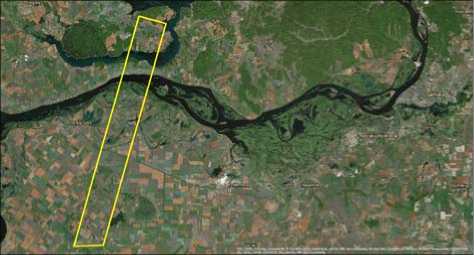
Fig. 1. Study area image, Samara region, Russia (source: Google Earth)

Field work and ground trothing

Fieldwork to map individual land cover classes and obtained spectral measurements of the dominant species was conducted at 60 sites in Samara region, Russia. Ground-trothing surveys should be undertaken within two weeks of acquiring satellite remote sensing imagery [10]. The winter field campaigns took place on 10 to 25 January 2017 and summer was on 15 to 30 August 2017. A random sampling method was used across the Samara region, around 7-8 samples selected in each class. The FieldSpec 3 ASD handheld spectrometer was used to obtain quantitative measurements of radiant energy easily and efficiently. We find 8 major and 27 sub-classes as shown in table 1.

Selection of satellite data

In this research work we consider spatial, spectral and temporal resolution as well as cost and availability of data, when we reviewing most appropriate data [11]. The Hyperion hyperspectral sensor (United States Geological Survey Earth Resources Observation Systems) and the multispectral Operational Land Imager (OLI) and Advance Land Imager (ALI) sensors [12] were then selected for this study. Few characteristics of all three sensors are representing in table 2.

Table 1. Land cover classes and their sub-classes in study area

Sr. No	Class level I	Class level II	Class level III
1.	Water	1.1. Inland water body	1.1.1 Deep water
			1.1.2 Shallow water
			1.1.3 Turbid water
			1.1.4 Clean water
		1.2 Lake
		1.3 River
2.	Vegetation	2.1 Forest	2.1.1 Conifer forest
			2.1.2 Deciduous/ Broadleaved forest
			2.1.3 Mixed forest
		2.2 Agriculture	2.2.1 Heterogeneous agricultural area
			2.2.2 Permanent crops
		2.3 Mangroves
		2.4 Grassland
		2.5 Sparsely vegetated area
3.	Settlements	3.1 residential	3.1.1 Old residential
			3.1.2 New residential
		3.2 Industrial
		3.3 Park
4.	Wetland
5.	Bare land	5.1 Scrubland
		5.2 Transitional woodland
6.	Transporta-tion	6.1 Road	6.1.1 Highway
			6.1.2 Inside road
			6.1.3 Concrete road
		6.2 Rail
7.	Bare rocks
8.	Sand dunes

Table 2. Characteristics of Hyperion, OLI and ALI sensors

Sr. No.	Characteristics	Values              1
		Hyperion	OLI	ALI
1	Sensor type	Pushbroom	Push-broom	Pushbroom
2	Wavelength range	400 – 2.50 nm	434– 1.38 nm	433 – 2.35 nm
3	Number of spectral bands	242	9	7
4	Spectral resolution	10 nm	15–200 nm	5 –30 nm
5	Spatial resolution	30 m	30 m	30 m
6	Swath	7.5 km	185 km	37 km
7	Digitization	12 bits	12 bits	12 bits
8	Altitude	705 km	705 km	705 km
9	Repeat	16 day	16 day	16 day

Collection of spectral measurements

Spectral measurements were made in the field from the forest area, agriculture field, mixed vegetation, different water bodies, river, highway, concrete road, railway line, sand dunes, rocks and wetlands etc. by the FieldSpec 3 ASD Spec-troradiometer. All data collected were georeferenced using real time differentially corrected GPS (Trimble PRO XRS) with 1 m accuracy, which allowed identifying specific pixels where field spectra were measured. A reconnaissance of all sites was completed with the help of local exports and samples were collected for all land cover classes for secondary identifications. FieldSpec 3 ASD Spectroradiometer device is an optical device that uses detectors other than photographic film to measure the distribution of radiation in a particular wavelength region; which measure the radiant energy (radiance and irradiance). It measures the spectral behavior in the visible, near-infrared (VNIR) and shortwave infrared (SWIR) spectra between 350 and 2500 nm in a precision of 1 nm.

Data preprocessing

Digital image processing was manipulated in ArcGIS software. The scenes were selected to be geometrically corrected, calibrated and removed from their dropouts. All images were projected in UTM 39N, datum WGS 84 projection. Other image enhancement techniques like histogram equalization were also performed in each image for improving the quality of the image. Some additional supporting data were used in this study such as filed data and topographic sheets. Digital topographical maps, 1:50,000 scale, were used for image georeferencing for the land use/cover map and to increase accuracy of the overall assessment [13]. Using ArcMap, we made a composite raster data of OLI and ALI using Arctoolbox data management tools. Both images were composed of 9 and 7 different bands respectively, each representing a different portion of the electromagnetic spectrum. By combining all these bands, composite raster data were obtained. Table 3 shows details of all three data.

Table 3. Left: Wavelength ranges of the OLI image. Right: Wavelength ranges of the ALI image.

OLI Bands	Wavelength (micrometers)	Resolution (meters)
Band 1 – Ultra Blue	0.435 – 0.451	30
Band 2 – Blue	0.452 – 0.512	30
Band 3 – Green	0.533 – 0.590	30
Band 4 – Red	0.636 – 0.673	30
Band 5 – Near Infrared (NIR)	0.851 – 0.879	30
Band 6 – Shortwave Infrared	1.566 – 1.651	30
Band 7 – Shortwave Infrared	2.107 – 2.294	30
Band 8 – Panchromatic	0.503 – 0.676	15
Band 9 – Cirrus	1.363 – 1.384	30
ALI Bands
Pan	0.48 – 0.69	10
MS – 1'	0.433 – 0.453	30
MS – 1	0.45 – 0.515	30
MS – 2	0.525 – 0.605	30
MS – 3	0.63 – 0.69	30
MS – 4	0.775 – 0.805	30
MS – 4'	0.845 – 0.89	30
MS – 5'	1.2 – 1.3	30
MS – 5	1.55 – 1.75	30
MS – 7	2.08 – 2.35	30

For pre-processing of Hyperion imagery, first georeferenced the image, subsequently were removed the noncalibrated bands of the Hyperion imagery (namely bands 1 – 7; 58–76; 77–78; 225–242). Hyperion VNIR spectrometer has 70 bands of which only 50 are calibrated, while the SWIR spectrometer has 172 bands of which only 148 are calibrated. The 198 calibrated bands cover the entire spectrum from 426 to 2395 nm (USGS, 2011). Also the Hyperion imagery water absorption bands (namely bands 120– 132, 165– 182, 185– 187, 221 – 224) were eliminated in order to reduce the data which influence by atmospheric scatter and water vapor absorption, caused by well mixed gasses. Bands 77 and 78 were also eliminated because they had a low SNR value and overlapped with band 56 and 57 respectively. In the next step, the Hyperion imagery bands with vertical stripping were identified based on visual inspection and those were manually removed (namely bands 8, 55–57, 79–82, 96–100, 120–134, 165–190, 220– 224). Vertical stripes are caused by differences in gain and offset of different detectors in push broom-based sensors such as Hyperion and vertical stripping are usually identified by visual inspection of the image data or atmospheric modeling. Then, the at-sensor radiance was computed from the raw Digital Number (DN) values, for all remained spectral bands. This was derived by dividing the pixel’s DN by a constant value, which was 40 for the visible and nearinfrared (bands 8–57) and 80 for the short-wave infrared (bands 79–224) (USGS, 2011). Atmospheric correction was not applied, as according to [13] ‘‘it is not necessary to atmospherically correct image data for a single observation’’. Also, taking into account that the Hyperion imagery was already terrain-corrected, no further correction for topographic effects deemed necessary.

Subsequently, a minimum noise fraction [15] was applied on Hyperion data set in order to separate noise from data and to minimize the influence of systematic sensor noise during image analysis, as it has been done previously by other investigators [16]. Hyperion final data set after the implementation of an inverse MNF consisted of 132 bands, 45 in the VNIR and 87 in the SWIR. After this step, the resulting image was reduced to a subset of the studied region. These final 132 bands after this last pre-processing step were used in the present study (fig. 2).

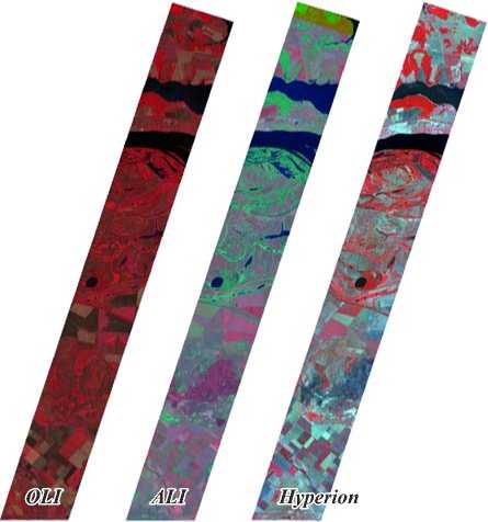
Fig. 2. A sub-scene of the geometrically corrected OLI, ALI and Hyperion image over the study area in Samara region, Russia

Classification

In this research work we use USGS land use/cover classification system for all three images (fig. 3). For all three images, k -nearest neighbor algorithm (KNN) supervised classification and migrating means clustering unsupervised classification (MMC) approach was applied [17]. Training sites were collected based on field data and also take help with topography maps. Initially, training sites were chosen for all 27 sub-classes derived from all three images, than all 27 sub-classes were aggregated into following 8 meager classes 1. Water; 2. Vegetation; 3. Settlements; 4. Wetland; 5. Bare land; 6. Transportation; 7. Bare rocks and 8. Sand dunes. For accuracy assessment 60 points were randomly collected in each image.

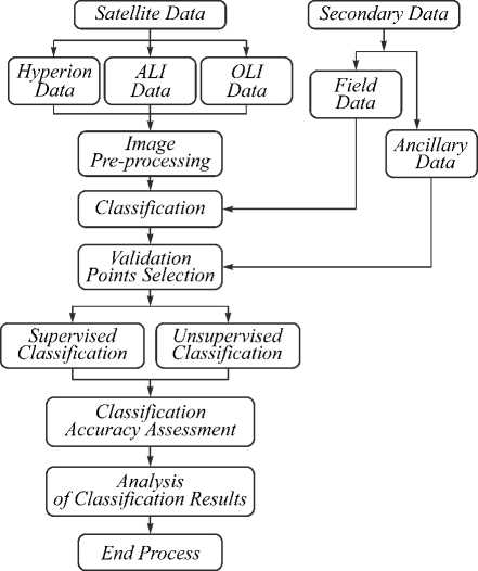
Fig. 3. Flow diagram of methodological process

Unsupervised classification

In unsupervised classification, image processing software classifies an image based on natural groupings of the spectral properties of the pixels, without the user specifying how to classify any portion of the image. Conceptually, unsupervised classification is similar to cluster analysis where observations (in this case, pixels) are assigned to the same class because they have similar values. The user must specify basic information such as which spectral bands to use and how many categories to use in the classification or the software may generate any number of classes based solely on natural groupings. Common clustering algorithms include K-means clustering, ISODATA clustering, and Narenda-Goldberg clustering.

Unsupervised classification yields an output image in which a number of classes are identified and each pixel is assigned to a class. These classes may or may not correspond well to land cover types of interest, and the user will need to assign meaningful labels to each class. Unsupervised classification often results in too many land cover classes, particularly for heterogeneous land cover types, and classes often need to be combined to create a meaningful map. In other cases, the classification may result in a map that combines multiple land cover classes of interest, and the class must be split into multiple classes in the final map. Unsupervised classification is useful when there is no preexisting field data or detailed aerial photographs for the image area and the user cannot accurately specify training areas of known cover type. Additionally, this method is often used as an initial step prior to supervise classification (called hybrid classification). Hybrid classification may be used to determine the spectral class composition of the image before conducting more detailed analyses and to determine how well the intended land cover classes can be defined from the image.

Supervised classification

In supervised classification the user or image analyst “supervises” the pixel classification process. The user specifies the various pixels values or spectral signatures that should be associated with each class. This is done by selecting representative sample sites of known cover type called Training Sites or Areas. The computer algorithm then uses the spectral signatures from these training areas to classify the whole image. Ideally the classes should not overlap or should only minimally overlap with other classes.

In ArcGIS software there are many different classification algorithms and we can choose any from supervised classification procedure as:

Maximum Likelihood: Assumes that the statistics for each class in each band are normally distributed and calculates the probability that a given pixel belongs to a specific class. Each pixel is assigned to the class that has the highest probability (that is, the maximum likelihood). This is the default.

Minimum Distance: Uses the mean vectors for each class and calculates the Euclidean distance from each unknown pixel to the mean vector for each class. The pixels are classified to the nearest class.

Mahalanobis Distance: A direction-sensitive distance classifier that uses statistics for each class. It is similar to maximum likelihood classification, but it assumes all class covariances are equal, and therefore is a faster method. All pixels are classified to the closest training data.

Spectral Angle Mapper: (SAM) is a physically-based spectral classification that uses an n -Dimension angle to match pixels to training data. This method determines the spectral similarity between two spectra by calculating the angle between the spectra and treating them as vectors in a space with dimensionality equal to the number of bands. This technique, when used on calibrated reflectance data, is relatively insensitive to illumination and albedo effects.

K-nearest neighbor algorithm (KNN): K nearest neighbors is a simple algorithm that stores all available cases and classifies new cases based on a similarity measure (e.g., distance functions). KNN has been used in statistical estimation and pattern recognition already in the beginning of 1970's as a non-parametric technique. Pattern recognition is the scientific discipline whose goal is the classification of objects into a number of categories or classes. Depending on the application, these objects can be images or signal waveforms or any type of measurements that need to be classified. We will refer to these objects using the generic term patterns.

In supervised classification the majority of the effort if done prior to the actual classification. Once the classification is run the output is a map with classes that are labeled and correspond to information classes or land cover types. Supervised classification can be much more accurate than unsupervised classification, but depends heavily on the training sites, the skill of the individual processing the image, and the spectral distinctness of the classes. If two or more classes are very similar to each other in terms of their spectral reflectance (e.g., annual-dominated grasslands vs. perennial grasslands), misclassifications will tend to be high. Supervised classification requires close attention to development of training data. If the training data is poor or not representative the classification results will also be poor. Therefore supervised classification generally requires more times and money compared to unsupervised classification.

Classification accuracy assessment

Accuracy assessment of the thematic maps produced from the implementation of the supervised and unsupervised classification techniques on Hyperion, ALI and OLI imagery was also performed in ArcGIS based on the confusion matrix analysis [18]. As a result, the overall (OA), user’s (UA) and producer’s (PA) accuracies and the Kappa (Kc) statistic were computed. The OA provides a measure of the overall classification accuracy and is expressed as percentage (%). OA represents the probability that a randomly selected point is classified correctly on the map. Kc provides a measure of the difference between the actual agreement between reference data and the classifier used to perform the classification versus the chance of agreement between the reference data and a random classifier. PA indicates the probability that the classifier has correctly labeled an image pixel. UA expresses the probability that a pixel belongs to a given class and the classifier has labeled the pixel correctly into the same given class. In performing the accuracy assessment herein, a total of 60 sampling points for the different classes were selected (approximately 25 pixels per class) directly from the imagery following a random sampling strategy, and these points formed our validation dataset. Selection of those validation points was performed following exactly the same criteria used for the selection of training points, described earlier (Section 3.3.2). For consistency, the same set of validation points were used in evaluating the accuracy of the land use/cover thematic maps produced.

Results and discussion

Developing the spectral library

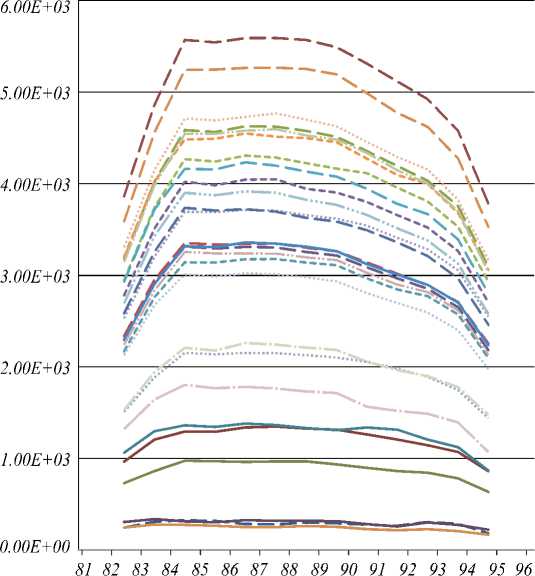
The land cover spectral library was developed by collected spectra of different sites from all three data sates and later on used as a set of reference spectra (fig. 4), to define different classes and mixed communities in Samara region, Russia. The average spectra illustrate a typical pattern, with significant divergence in the shape of the spectral curve between different land cover classes. The resulted spectral library shows all land cover class separation is possible in infrared region for all three data. In compare of all three datasets, all classes can easily separate in Hyperion data, as it have continues spectral band with very narrow bandwidth so specific bandwidth is sensitive for specific land cover class. ALI and OLI data have less capacity to separate all land cover class in compare of Hyperion data due to less number of bands and longer bandwidth (fig. 4). In compare of ALI and OLI data sets, ALI has better results due to specific quality of sensor.

In Hyperion data in visible range from band number 8 to 31 only major land cover classes were define and subclass level separation is not possible but in infrared region from band number 35, all land cover classes were easily separate, even till sub-class levels. In infrared region lowest reflectance was from river water and later on clean, shallow and turbid water, which show clear and deep water absorbed by IR range and once it’s shallow or turbidity increase, its reflectance was increase. In the study region lake water have highest reflectance, it means lake water is shallow with high turbidity. ALI data also show same thing like Hyperion but in OLI data reflectance difference is very less in all type of water categories. Therefore, we can identify water classes in EO -1 (Earth Observing 1) Hyperion and ALI both data but not in Landsat OLI data.

For the vegetation in the visible range of Hyperion data, reflections were low due to photosynthetic pigment absorptions except for the low peak in the green wavelengths. Reflectance was highest in the near-infrared between 700

and 1300 nm, due to lack of strongly absorbing materials in plants in this region of the spectrum. A strong absorption feature was found around 1450 nm, caused by water in the canopy. There were smaller water absorptions around 970 nm and 1140 nm. Species can be identified based on shape differences that were present across the spectrum. Regardless of which site the spectra were measured, different samples of the same species produced spectra within a limited range of variation. The consistency may have benefited from the measurements being made on mature canopies in discrete patches in Hyperion data. In vegetation deciduous forest have highest reflectance then mangroves, sparsely vegetated area and in last permanent crops in Hyperion data. In ALI data in IR range permanent crops have highest reflectance then mangroves, mixed forest, deciduous forest, sparsely vegetated area, heterogeneous vegetated area and in last grassland. In Landsat OLI data mangroves have highest reflectance then, deciduous forest, heterogeneous agriculture area, permanent crops, sparsely vegetated area, grassland and in last mixed forest.

In Hyperion data old residential areas (settlements) have high reflectance than industrial area, new residential area and in last parks. In ALI and OLI image parks have highest reflectance then industrial area, old and in last new residential area. For transportation in Hyperion and ALI data, the reflectance was highest from highway, then inside road, rail and concreate road and for OLI data highest reflectance from concreate road, then rail, inside road and highway. Other land cover classes reflectance based on water content as wetland is always very close reflectance to water classes and bare land has high reflectance. Send dunes have high reflectance then rocks in IR region due to vegetation coverage (fig. 4).

1.1.1

1.1.2

1.1.3 1.1.4

1.2

1.3

2.1.1

2.1.2

2.1.3

2.2.1

2.2.2

2.3

2.4

2.5

3.1.1

3.1.2

3.2

3.3

5.1

5.2

6.1.1

6.1.2

6.1.3 6.2

Deep water

Shallow water

Turbid water

Clean water

Lake

River

Conifer forest

Deciduous forest

Mixedforest

Heterogeneous agricultural area

Permanent crops

Mangroves

Grassland

Sparsely vegetated area

Old residential

New residential

Industrial

Park

Wetland

Scrubland

Transitional woodland

Highway

Inside road

Concrete road

Rail

Bare rocks

Sand dunes

Fig. 4. Representative spectra for 27 land cover classes by Hyperion data from band number 82 to 96 in Samara, Russia

Samara region land cover classes were defined into 8 major and 27 sub-classes based on species abundances and the characteristic dominant and sub-dominate land covers. For purposes of building the spectral library, a good understanding of the all land cover classes at each location in the study area was needed to utilize fully the information content of the spectra. Intra-specific and intracommunity variation were found across disturbance gradients. Phenomena included pattern, shape-size, water content, structural changes, reduced biomass, lower “greenness” and chlorophyll, chlorosis and corresponding shifts across the spectral response curve. Methodological approaches to account for this variability, which can be used to assess stress, are still to be resolved. Large sets of reference spectra may be needed to fully characterize this variability. However, in this study, some land cover classes have similar spectral signature in different locations give additional benefits to sub-class level or species level mapping without a priori knowledge. However similar reflectance of mixed classes create confusing and difficult to identify class without field data or additional testing of spectral unmixing and other spectral matching techniques.

Using spectral library for land cover classification

Simple land use/cover classes such as forest, agriculture, settlements, water body and bare land can easily classify in high resolution data, even for their classification, we no need to use spectral library. Fig. 5 show Normalized Difference Vegetation Index (NDVI) images for all three data sets and in these images major land cover classes such as vegetation, water etc. can easily identify. As distinct land cover class patterns are closely related with specific bands/channels so without field data or spectral library or site situation/condition, these patterns cannot be identify, so basically, we need spectral library for sub-class level land cover classification.

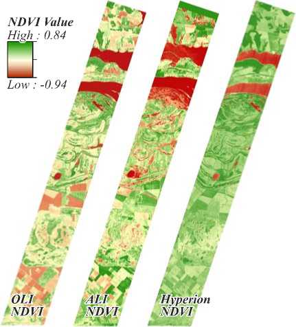
Fig. 5. Biomass and biochemical variation are readily discernable in the Normalized Difference Vegetation Index (NDVI) in all three satellite data

A land cover map based on spectral library on hyper-spectral (Hyperion) and multispectral data (OLI, ALI) produce 27 land cover classes (fig. 6).

In comparison, hyperspectral data provide better results in place of multispectral data. This finding is similar to [19], who found that spectral resolution was more important for correct classification than spatial resolution, except in cases where high within pixel heterogeneity exceeded the pixel-to-pixel variance. In this research work a similar classification was produced from reference spectra extracted from the image (using GPS coordinates to identify classes) as from field-measured spectra of those land cover classes and resulted land cover map is a good representation of spectral pattern change due to continuous spectral bands in hyperspectral data.

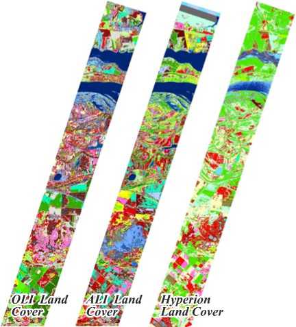
Land Cover Classes

M 1.1.1 Deepwater

■ 1.3 River

□ 6.2 Rail            □ 2.1.1 Conifer forest

■ 2.1.2 Deciduous Forest □ 6.1.2 Insideroad

□ 1.1.4 Clean water □ 5.1

□ 1.2 Lake □ 2.2.1

□ 1.1.2 Shadow water

□ 1.1.3 Turbid waler □ 2.3

□ 6.1.3 Concrete road □ 5.2

□ 4 Wetland

Scrubland Heterogeneous agricultural area Mangroves Transitional woodland

Mixed forest Sand dunes

□ 3.1.2 New residential

□ 7   Bare rocks   □ 2.1.3

□ 6.1.1 Highway    □ 8

Industrial

Old residential

Park

Sparsely vegetated area

Grassland

Permanent crops

Fig. 6. Land cover map derived with the combined spectral library of OLI, ALI, Hyperion images and field based observations over the study area

Now we can say for wider use of hyperspectral data require improved methodologies and tools that facilitate and automate basic analyses and mapping, that can be specifically applied to land cover requirements.

Both field and image methods for obtaining reference library spectra required complex processing and analysis. If a standard spectral library for land cover classes/ communities can be developed, it will aid resource managers by allowing them to utilize newer more powerful image analysis techniques while avoiding the data processing and expertise required to create the database. [20] similarly concluded that key challenges in applying these technologies on a wider scale included: building human capacity in advanced science and technology-based approaches, de- velopment of low cost and rugged IR spectroscopy instrumentation and development of decision support systems to help interpret spectroscopy data.

Classification comparison

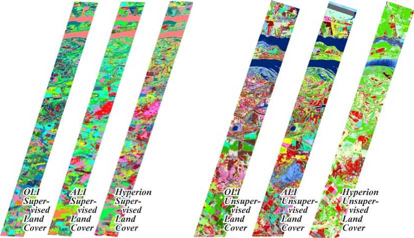
The LULC maps produced by supervised and unsupervised classification on Hyperion, ALI and OLI data acquired over the study region are demonstrated in fig. 7.

The statistical results of classification accuracy assessment are shown in table 4. On the basis of accuracy assessment results, its appear that supervised classification somehow better results than unsupervised classifica- tion in overall accuracy and individual classes accuracy. Results indicate that for KNN the overall accuracy was 95, 94, 88 and kappa coefficient .91, .89, .85 for Hyp, ALI, OLI respectively, whereas for unsupervised it was 93, 90, 84 overall accuracy and .89, .87, .81 kappa coefficient for Hyp, ALI, OLI respectively. Among the two classifiers, supervised classification was the best in describing the spatial distribution and the cover density of each land cover category, as was also indicated from the statistics of the individual classes’ results produced (table 4).

□ 1.1.1

□ 1.1.2

□ 1.1.3

■ 1.1.4

□ 1.2

■ 1.3

□ 2.1.1

□ 2.1.2

■ 2.1.3

□ 2.2.1 □ 2.2.2 □ 2.3 □ 2.4 ■ 2.5

□ 3.1.1

■ 3.1.2 ■ 3.2 □ 3.3

□ 4

■ 5.1

■ 5.2

□ 6.1.1

■ 6.1.2

■ 6.1.3

□ 6.2

□ 7

■ 8

Land Cover Classes

□ 6.2 Rail

■ 2.1.2 Deciduous Forest

□ 5.1  Scrubland

□ 2.2.1 Heterogeneous agricultural area

■ 2.3  Mangroves

□ 5.2  Transitional woodland

□ 2.1.3 Mixed forest

□ 8 Sand dunes

□ 2.1.1 Conifer forest

□ 6.1.2 Insideroad

□ 3.1.2 New res iden tial

□ 3.2 Industrial

□ 3.1.1 Old residential

□ 3.3  Park

■ 2.5  Sparsely vegeta ted area

□ 2.4 Grassland

□ 2.2.2 Permanent crops

1.1.1 Deepwater

1.3 River

1.1.4 Clean water

1.2 Lake

1.1.2 Shadow water

1.1.3 Turbid water

6.1.3 Concrete road

4    Wetland

7    Bare rocks

6.1.1 Highway

Fig. 7. OLI, ALI and Hyperion images classified land cover maps by supervised and unsupervised classification methods

In all classes similar patterns were easily identify in both classification. PA and UA for the supervised classification ranged between the classes from 86% to 99 %, and from 79% to 94%, whereas for unsupervised classification varied from 82% to 95 % and from 75 % to 92 % respectively.

In both classification the highest accuracy were in turbid water, permanent crops, sparsely vegetated area and bare rocks classes, followed by deep water, industrial, mixed forest, grassland, highway and sand dunes classes. In individual classes the lowest PA and UA in both classifications were shallow water, clean water, turbid water, grassland and highway classes.

For all three data the highest PA and UA present in Hyperion data and lowest value present in OLI data. This was perhaps due to the similar spectral characteristics between the two classes, which was affected by the mixed pixels, caused by the low density of these vegetation types and combined with the low spatial resolution of the sensors.

So overall we can say supervised classification is better than unsupervised classification. In unsupervised classification algorithms require the analyst to assign labels and combine classes after the fact into useful information classes (e.g. forest, agricultural, water, etc). In many cases, this after the fact assignment of spectral clusters is difficult or not possible because these clusters contain assemblages of mixed land cover types. Generally speaking, unsupervised classification is useful for quickly assigning labels to uncomplicated, broad land cover classes such as water, vegetation/non-vegetation, forested/non-forested, etc). Furthermore, unsupervised classification may reduce analyst bias. But supervised classification allows the analyst to fine tune the information classes--often too much finer subcategories, such as species level classes. Training data is collected in the field with high accuracy GPS devices or expertly selected on the computer. Consider for example if you wished to classify percent crop damage in corn fields. A supervised approach would be highly suited to this type of problem because you could directly measure the percent damage in the field and use these data to train the classification algorithm. Using training data on the result of an unsupervised classification would likely yield more error because the spectral classes would contain more mixed pixels than the supervised approach. Simi- larly, collecting in the field crop species training data is preferable to expertly selecting pixels on screen, as it is often very difficult to determine which crops are growing visually.

That`s why supervised classification is outperformed the unsupervised classification. When we compare both classification in hyperspectral and multispectral data, results show that supervised classification have highest accuracy, which authors attributed to the supervised ability to locate an optimal separating hyperplane.

Table 4. Summary of the results from the classification accuracy assessment conducted

Land cover classes	Supervised Classification						Unsupervised Classification
	Producer’s accuracy (%)			User’s accuracy (%)			Producer’s accuracy (%)			User’s accuracy (%)
	Hyp	ALI	OLI	Hyp	ALI	OLI	Hyp	ALI	OLI	Hyp	ALI	OLI
1.1.1 Deep water	98	91	88	90	83	84	95	86	85	88	80	81
1.1.2 Shallow water	94	93	86	87	86	78	92	90	82	85	81	75
1.1.3 Turbid water	99	93	87	91	86	79	94	90	84	90	82	76
1.1.4 Clean water	95	92	87	87	86	78	91	87	83	86	83	75
1.2 Lake	95	93	87	87	85	82	90	91	82	84	81	80
1.3 River	91	93	88	85	88	80	88	90	85	81	85	79
2.1.1 Conifer forest	94	93	88	89	86	82	89	89	86	84	82	80
2.1.2 Deciduous/ Broadleaf forest	92	99	92	83	92	86	90	96	90	80	90	81
2.1.3 Mixed forest	92	97	92	84	91	86	91	94	90	81	89	82
2.2.1 Heterogeneous agricultural	94	92	90	87	86	81	90	87	89	83	82	80
2.2.2 Permanent crops	99	92	90	94	88	85	95	88	89	92	85	81
2.3 Mangroves	96	93	91	91	88	87	92	90	90	90	83	85
2.4 Grassland	95	97	88	89	91	79	91	94	85	86	90	76
2.5 Sparsely vegetated area	99	92	88	91	84	82	96	88	84	90	81	81
3.1.1 Old residential	95	94	86	90	88	81	91	90	82	89	83	80
3.1.2 New residential	94	94	87	85	85	80	90	90	84	82	80	77
3.2 Industrial	98	94	89	93	88	85	95	91	86	91	84	81
3.3 Park	93	93	87	88	85	81	90	90	85	86	81	78
4. Wetland	94	93	88	86	88	80	91	90	84	84	86	79
5.1 Scrubland	96	92	88	89	88	81	91	89	84	85	85	78
5.2 Transitional woodland	95	92	95	87	85	85	90	90	92	83	80	82
6.1.1 Highway	94	97	87	89	91	79	89	94	84	86	90	76
6.1.2 Inside road	92	99	87	86	94	81	88	95	83	82	91	80
6.1.3 Concrete road	93	92	86	85	86	81	87	89	82	81	82	77
6.2 Rail	96	96	87	86	86	81	90	91	82	81	81	79
7. Bare rocks	99	94	88	94	86	83	94	90	85	91	83	81
8. Sand dunes	95	97	88	89	88	84	91	92	86	86	86	82
Overall accuracy	95	94	88				93	90	84
Kappa coefficient	.91	.89	.85				.89	.87	.81

Conclusions

This research work demonstrates the potential of hy-perspectral and multispectral data for land cover monitoring and assessment. Currently, limitations of both data availability and cost remain, as do significant methodological and technical issues. However, this research work highlights developing spectral library for land cover classes. In order to facilitate a global approach to applications of new advanced technologies for mapping and monitoring of landscape, a standardized classification system for land cover classes should be adopted to make best use of the spectral libraries and to facilitate a global remote sensing-based monitoring and assessment capacity. Additionally spectral library provide useful reference framework for landscape assessment, also support, and promote new technology in terms of new space based high-resolution hyperspectral instruments for earth observation. The accuracy assessment results show that supervised classification is better than unsupervised classification for all three (Hyperion,

ALI and OLI) imagery. The higher classification accuracy reported by supervised classification is mainly attributed to the fact that this classifier has been designed as to be able to identify an optimal separating hyperplane for classes’ separation, which the unsupervised may not be able to locate. This research found that, data analysis of hyperspectral imagery has the potential for improving classification accuracies of land cover and land use over multispectral imagery with the same resolution. If images were acquired the same day and time, then accuracies would be even more comparable. The latter, from an operational perspective, can be of particular importance particularly in the Mediterranean basin, since it can be associated to the mapping and monitoring of land degradation and desertification phenomena that are frequently pronounced in such areas.