Comparison of Two Methods Basing on Artificial Neural Network and SVM in Fault Diagnosis

Published Online November 2010 in MECS

In a power system, power electronics particularly subject to constant stress of over-current surge and voltage swings because they normally operate in an environment requiring rapid speed variations, frequent stop and constant overloads. Although protection devices such as snubber circuits are commonly used, switching devices are physically small thermally fragile. Moreover, even a small electrical disturbance can cause thermal rating to be exceeded, resulting in rapid destruction of the device [1]. In many expensive, high-power systems, multi-converter integrated automation systems and safety critical systems, any unusual performance may lead to sudden system failure [2]. So fault diagnosis for those power electronics is necessary.

This letter presents a diagnosis method for a pulse width modulation (PWM) voltage source inverter shown in Fig.1. Two methods basing on artificial neural network classifier and SVM are proposed to detect and identify the transistor open-circuit fault. The structure of BPNN is simple and it is capable of recognition. However, it has several shortcomings obviously. Namely: low convergence rate, local minimum, and complicity of hidden layers.

The rest of the paper is organized as follows:

Firstly, background on the ANN and SVM is introduced in this article. Next, system simulation is presented. Then, two methods basing on neural network and SVM are proposed to detect SPWM inverter. Finally the conclusions and comparison are shown.

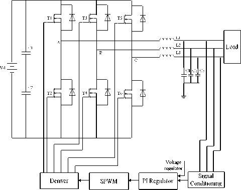
Figure 1. PWM voltage fed inverter

• II.    BACKGROUND

In the past two decades, the techniques of neural network have grown mature as a data-driven method which provides a new perspective to fault diagnosis. There are basically two ways to approach the analytical fault detection problem. That is the model-based approach and the data-based approach. The latter bypasses the step of obtaining a mathematical mode and deals directly with the data. This is more appealing when the process being monitored is unknown to be linear or when this is too complicated to be extracted from the data [3]. Therefore the purpose of using ANN is the realization of nonlinear functions which can estimate a suitable output from any inputs after training with a sample dataset.

SVM has its roots in statically learning theory and has shown promising empirical results in many practical applications, from handwritten digit recognition to text categorization.

A linear SVM is a classifier that searches for a hyper plane with the largest margin, which is why it is often known as a maximal margin classifier.

Advantages of SVM:

• (1)    Good at high dimensional problems

• (2)    Up to global optimum. Not like the other rule based classifiers and neural network who employ greedy-based strategy to search the hypothesis space. Such methods tend to find only locally optimum solution.

  
  

  -^-2¹0⁰0⁰⁰

  -200

  
  

  III. S YSTEM SIMULATION

  
  

  MATLAB is used to simulate the inverter for training and test the proposed scheme. All kinds of open-fault of transistor can be identified by it.

  
  

  -300

  
  

  0.01

  
  

  0.02

  
  

  0.03 t(s)

  
  

  0.04

  
  

  0.05

  
  

  0.06

  
  
  

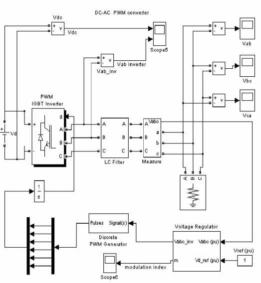
  Figure 2. Simulation of three-phase SPWM convertor

  
  

  Figure 4. Transistor T1 open-circuit fault

  
  

The first open-fault of transistor T1 is introduced and features will be extracted from its voltage waveforms. Fig.2 and Fig.3 respectively display the voltage waveforms of T1 when it is free fault and happens to open-fault.

Short-circuit fault and open faults are vulnerable in power electronic circuits, and this article only SCR fault diagnosis are discussed.

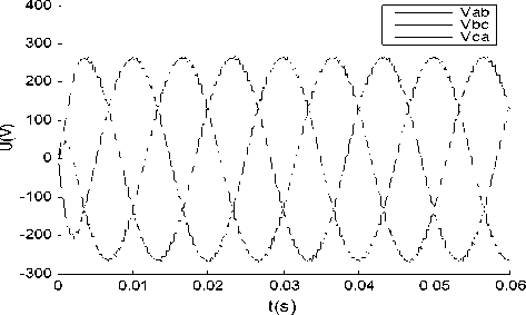
Figure 3. Transistor T1 free fault

The output voltage of the same or similar shape, but different timeline between the corresponding waveform fault states are divided into the same class. the normal state as a special kind of failure to consider the time, and only two SCR faults are considered, failure can be divided into 5 categories, 22 Class.

The first category: free-fault.

The second category is single fault, which includes: T1, T2, T3, T4, T5, and T6.

The third category is two IGBT faults of same phase, which includes: T1T2, T3 T4, and T5T6.

The forth category is two IGBT fault of same half-bridge, which includes: T1T3, T2T4, T3 T5, T4 T6, T1T5, T2T6.

The fifth category is two IGBT fault of cross, which includes: T1T4, T2T3, T2 T5, T1 T6, T3T6, and T4T5.

• IV. NEURAL NETWORK CLASSIFIER

The fault detection can be divided into four main stages: sense of fault, preprocessing and feature extraction; design of neural networks; networks optimization; fault discrimination using ANN.

• A.    feature extraction by FFT

  

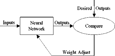
  Figure 5. Model of a neural network

  
  

The time domain waveform signal can be converted into frequency domain analysis through Fast Fourier Transform. We choose dc component, fundamental amplitude, and phase, the second harmonic amplitude and phase, and the third harmonic phase as features. Those selections can offer better results. The feature vectors are fed to the BPNN as training data or testing data.Table1shows some training samples.

TABLE I.

SOME TRAINING SAMPLES

Circuit stage	D 0	A 1	ϕ 1	A 2	ϕ 2	ϕ 3
free-fault	3.97	169.50	26.60	9.80	240.40	229.90
T1	54.54	105.20	45.10	29.27	89.50	246.20
T2	49.22	100.50	46.30	42.44	266.70	244.00
T3	40.99	117.20	6.40	20.24	0	0
T1T2	4.04	77.97	92.90	6.02	250.80	0
T3T4	0.25	83.30	0	2.70	118.10	33.10
T5T6	3.02	165.10	27.40	6.82	249.10	210.80
T1T3	6.84	44.60	18.50	34.36	53.40	51.80
T4T6	64.65	88.77	10.70	22.49	129.20	0
T1T5	60.18	83.02	39.90	26.06	135.60	203.90
T2T6	58.42	75.82	44.20	29.31	0	231.00
T1T4	74.06	82.20	24.40	11.06	104.90	233.90
T2T3	72.62	76.03	25.40	18.38	265.20	257.70
T4T5	31.73	105.80	15.70	48.00	170.90	180.20

• B.    Design of neural network structure

An ANN pattern recognition scheme is developed to identify the weak points based on FFT features. Standard back propagation is a gradient descent algorithm, in which the network weights are moved along the negative side of adjusting weights and biases [2]. Fig.5 shows the model of a neural network [3].

We can conclude that ANN is trained to perform pattern recognition by adjusting the connection weights to find out the mapping relationship of input feature vectors and their corresponding target vectors.

The architecture of the BPNN model used in this study is three-layered. Each layer is represented as an input, middle, or output layer. The input layer receives data into a node .The node is a memory of a real number and its value is transmitted to another node by a connection. The middle layer is a data processor that transforms data and sends the transformed data to the output layer. The output layer is a display of the result by the ANN. After several adjustments, BP neural network structure is identified 6-21-6.Hidden layer activation function is Sigmoid function and output layer activation function is Pureline function.

TABLE II.

SOME T ESTING SAMPLES

Circuit stage	D 0	A 1	ϕ 1	A 2	ϕ 2	ϕ 3
T1	58.85	114.60	44.40	32.26	88.20	237.50
T2	52.47	109.60	45.70	49.98	263.50	234.00
T3T4	0.12	90.61	0	0.01	115.90	30.30
T1T3	7.88	48.77	16.60	37.19	50.20	45.70
T2T4	3.97	47.92	16.60	44.65	221.10	46.00
T4T6	69.36	95.95	9.90	25.72	125.90	0
T1T5	65.12	90.26	38.60	29.39	133.10	200.10
T2T6	63.26	81.43	42.50	33.27	0	226.50
T1T4	79.23	89.39	23.80	12.85	106.30	231.00
T2T3	77.96	81.33	24.60	21.70	263.70	252.40
T2T5	44.48	114.30	32.00	47.76	0	73.50
T1T6	50.28	117.00	33.70	34.28	110.10	36.70

• C.    Results

There are 122 training samples and 44 testing samples. Table 1 and table 2 are part of training samples and testing samples separately.

In practice, when hidden nodes are less than 13, the neural network is difficult to learn to converge to the required error. Considering the training time, network complexity and generalization, hidden nodes is 21 in a SPWM voltage inverter fault diagnosis.

TABLE III.

D IAGNOSIS RESULTS OF A TEST SAMPLES WITH NEURAL NETWORK

Category	Neural network output						expected output
free-fault	0	0.49	0.83	0.09	0.29	0.37	001000
T1	-0.01	1.03	-0.06	0.05	-0.08	0.94	010001
T2	-0.05	1.06	-0.01	-0.03	1.06	0.07	010010
T1T2	0	0.97	0.99	-0.03	0.03	0.99	011001
T1T3	1.01	-0.08	0.05	-0.01	-0.02	0.96	100001
T2T4	1.00	-0.02	0.06	0.02	1.02	0.11	100010
T3T5	0.90	0.09	0.02	0.09	0.98	1.12	100011
T1T4	1.01	-0.04	0.99	-0.04	0	1.05	101001
T2T3	0.94	0.02	1.08	-0.07	1.04	-0.03	101010
T2T5	1.01	0.11	1.24	-0.30	1.36	1.04	101011
T1T6	1.09	-0.19	0.96	1.27	-0.28	-0.23	101100
T3T6	1.01	-0.02	0.94	0.96	-0.01	1.04	101101
T4T5	0.99	0.08	0.97	1.04	1.03	0.10	101110

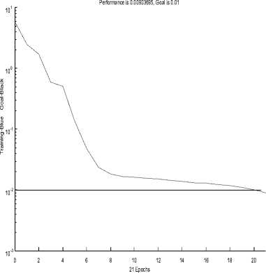
Figure 6. Convergence curve of BP algorithm

• V. SVM CLASSIFIER

• A. Linearly separable problems

SVM is developed from the optimal linear classification. Vapnik and others proposed this theory, which based on the principle of structural risk minimization of statistical learning. We illustrate the principle of SVM with two classifications in Figure6.

Training samples:

{ x n , У п } , x, e R^d , y. e { + 1, - 1}, i = 1,2, L n

Usually neural network design consists of input layer, hidden layer and output layer neuron number of the design. As to diagnosis of specific circuits, the input layer neurons and output layer neurons are decided by the specific issues. Their numbers are corresponding determined by the dimensions of the fault circuit and the number of the failure mode.

The difficulties are determination of the number of hidden neurons. Too few hidden nodes, the network convergence is not easy. But too many hidden nodes, then on the one hand this will increases the training time; the other hand, it is easy to fit the network. Thereby this may reduce the network's generalization ability. Commonly Minato test method is used to determine the number of neurons in hidden layer.

The learning process of the network error convergence curve can be seen from the figure6.The learning process neural network output error decreases, and the network calculation after 21 iterations to achieve the desired error, the curve convergence, then store the weights and thresholds, and will be testing samples to test the input neural network to get a diagnosis.

H 1 : w ■ x ₁ + b = + 1

H ₂ : w ■ x₂ + b = - 1

The distance of H1 and H2:

w 2

IIwll(x x ) = IN g (x ) = w ■ x + b = 0

G(x) can separate these samples,

,T 1 fw ■ x + b > 1 y,=+1Г 1

Namely: j            ‘    ^y,[w■ x,+ b]-1 > 0

^ w ■ x + b <  1 y i = -1

Any inputs, classification results are

У = sgn [ g ( ^x ) ]

+ 1

- 1

g ( x ) > ⁰

g ( x ) < ⁰

The maximum interval is equivalent to w ² minimum. Optimal hyper plane is the hyper plane requires not only separate the two, and make the classification of the largest interval, the former is to ensure that ERM, which is the generalization of the confidence interval to the minimum, so that the real risk minimization. In this way, the problem of classification

comes down to the following quadratic programming problem min 11 Iwl 12 =1 (w ■ w)

< w 211 2 (      )

s . t . y , ( w ■ x , + b ) > 1, i = 1,2, L n

n max W («) = Xa,- X yyaa (x, ■ xj)

= 1           ² , , j = 1

s.t.    Xa,y,= 0,a, > 0,1 = 1,2,L n(14)

= 1

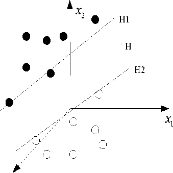
Figure 7. Optical dividing line under linear separable situation

The quadratic programming problem has a unique minimum point, so we use optimization theory in the Lagrange optimization algorithm.

n

^L ( w , b ^{, a} )=t ||w|| ^-X a [ y , ( ^w ■ x ⁺ b ) ^- 1 ]          ⁽⁷⁾

²             1 = 1

• a , : Corresponding Lagrange coefficients of each sample. Solution of the problem is decided by the Lagrange function saddle point, and this function must be minimized at w and b , for surely maximized at a .

dL     ^ =w -X a,y,x, =0 dw      1=1 (8) dL — = -? ay, = 0 5 b    1:7 (9) Solution is w = Xn a y x =1 (10) Xn a y =0 =1 (11) So nn

^L ( w . b . « ) = X а , - X yy a^ j (x,- x j )      ⁽¹²⁾

i = 1           ² 1 , j = 1

Tn

If a * = a, , a, L a „ I is solution, w * = Уа,у, x, 1     2, n

= 1

According to KKT principles a,*[y,(w*■ x) + b]-1 = 0 i=1,2,L n           (16)

Typically, only a small part of a , is not zero, the Corresponding sample is the support vector. Suppose 0 <  a , ' <  C is a component of a , .

From (16) we know nn b'=—- X y,a,‘ (x,x*)=y,- X y,a,’ (x,x*)

a,      ,=1

The optimal classification plane is

n

X a,* y,( x' x)+b *=0

= 1

Classification decision function g (x ) = sgn [X a,* y( Vx) + b * ]

• B. L nearly nseparable problems

nnn l (w,b,a)=Xa,- XXa^jy,yj^(x,)ф(xj)

= 1          ² , = 1 j = 1

If k (x, ,xj ) = ф (x, )■ ф (xj) , we can get the dual representation of the linear inseparable problem max q(a) = Xn^a,-1 XlILyyaa, k(x,,xj) a                        ,=1          2 ,=1 j=1

^

s . t . X a , y , = 0, 0 ^ a , <  C , "=1,2, L n t «                                     (21)

Suppose a * = [ a * , a ₂ * L a n ] T is solution, and 0 <  a , ‘ <  C is a component of a .we can obtain the nonlinear classification decision of the original space.

g ( x ) = sgn [^ L ^a , y , k ( x' ^x ) ^{+ b} ]                   ⁽²²⁾

C. Results

From dual principles, (12) is transformed into

LIBSVM is developed and designed by Chih-Jen Lin of Taiwan University. It is a simple, easy to use, fast and effective generic SVM software package that can solve the C-SVC classification, n-SVC classification, including one-algorithm-based multi-class pattern recognition problem; e -SVR regression, n -SVR regression; distribution estimation (one-class-SVM) and so on.

the introduction of Optimal classification interval and kernel function overcome the "curse of dimension" and "over-fitting" and other inevitable problems of traditional algorithms. Therefore, SVM is increasingly concerned by researchers. It has been initially demonstrated its performance is better than existing methods. Some scholars believe that SVM may become a new hotspot after neural network, and effectively promote the machine learning theory and technology.

• (1)    Selecting samples

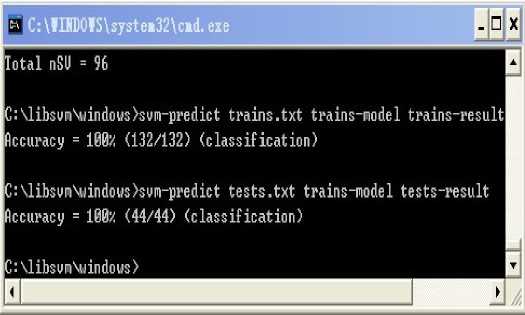
We use the same training data and test data as the neural networks in order to easily compare neural network and support vector machines advantages and disadvantages .There are 132 Training samples and 44 test samples in all. Those samples are from 22 species of SPWM inverter circuit failure. The dimension of each sample is 6.

• (2)    Scaling samples

The range of all samples can scaled into [ - 1,1 ] by svm-scale under specific rules.

• (3)    Training samples

After training samples, we can obtain The SVM model, as is shown in figure 8.

(5) Optimization parameters c and g

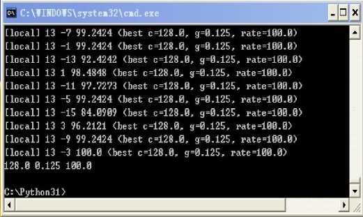
The last line is the optimal parameters.

Namely:

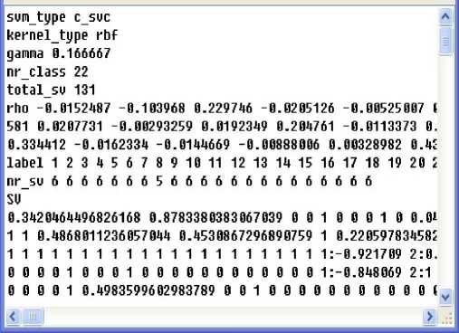
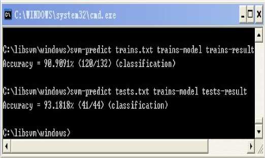
(4) Testing samples

c = 128, g = 0.125

(5) Re-training the test samples with the optimal parameters

VI. CONCLISION

It was concluded that SVM method offers better performance for power electronics and high availability than neural network. It can offer higher detection efficiency and reliability.