Compressive Sensing based Image Reconstruction Using Generalized Adaptive OMP with Forward-Backward Movement

Published Online October 2016 in MECS

Conventional image acquisition and reconstruction process consider the signal as a whole prior to dimensionality reduction via transform codes. Compressive sensing breaks this constraint of the traditional Nyquist Shannon theorem. It takes complete advantage of sparse signal in order to achieve the accurate recovery of the compressed signal. Compressive sensing is suggested by D. Donoho [1], E. Candes and T. Tao [2]. Compressive sensing makes high dimensional signal acquisition easy by combining sampling and compression [3]. The measured value is lesser as comparison to the amount of data that the traditional processes required. Compressive sensing firstly requires sparse signal having lower dimensions. The sparse signal contains maximum information with lesser number of captured observations. The implementation of CS method enables the reduction in the requirement of saving the majority amount of data which is actually not needed. Various fields exhibit the usage of CS theory in their implementation. The Classical methods for sparse representation include Fourier transform (FT), discreet cosine transforms (DCT), and discreet wavelet transforms (DWT) and etc. The methodology requires compressed observations via measurement matrix ( Φ ). Let us consider X is a signal in ℝN and it contains at most К≪N nonzero components. Here, x can be converted into sparse form by representing it in terms of orthonormal basis of N×1vectors {^i } as given:

X ⁽ t )=∑"=1 Si ^1 ( t ) (1)

where s is the sparse coefficient of X , S[ = ‹ X , Ф _i›. Here, s contains K nonzero components and hence called sparse signal, s is the sparse expansion of signal f in orthonormal domain. And, further the sparse signal is recovered with measurement process. In this methodology, measurement matrix Φ ∈ ℝ^{M x N} measures the71-dimensional signal and constructs the measurement vector У ∈ ℝ^M.

У =Φ x (2)

The measurement matrix is also known as measurement dictionary and each column in a normalized form is known as atom. Candes and Tao [2, 4] have suggested independent and identically distributed Gaussian random measurement matrix as an effective measurement matrix in compressive sensing. After obtaining у , the aim of recovery algorithm is to reconstruct the sparse signal х using У and Φ . The reconstruction problem is an ill-posed problem and requires stable and effective algorithms. The recovery algorithms are the major concern in compressive sensing. There are various recovery algorithms for CS paradigm. They can be generally classified into the following categories viz. Greedy Pursuit [5, 6, 7], Convex relaxation [4, 8] and Bayesian methods [9,10].The latter two methods are theoretically refined but computationally complex. On the contrary, Greedy pursuit algorithms are simple and require lesser number of measurements. Convex relaxation process uses ℓ i minimization instead of using ℓ 0 minimization for example Basis Pursuit (BP).Greedy Pursuit algorithm uses iterative technique such as Matching Pursuit (MP) [5], Compressive sampling MP (CoSaMP) [11], Orthogonal Matching Pursuit (OMP) [12], Iterative Hard Thresholding [13, 14], Generalised OMP (GOMP) [14] and Subspace pursuit (SP) [16]. In this paper, proposed Generalised adaptive OMP algorithm with forward-backward movement is presented that can recover the image accurately. The algorithm selects alternatively the number of atoms with forward backward movement. The movement allow the forward identification and backward removal steps. It expands the support estimate and compressed it simultaneously. The proposed algorithm works adaptively as the size of the selection set for forward and backward movement changes if certain conditions are met. It provides an advantage of performing better in most scenarios where lesser number of measurements is required. It can provide better results even if the priori estimate of sparsity K is not known [17].

The paper is structured as follows: A short description of related previous work is explained in Section II. Greedy pursuit techniques is presented for explaining conventional OMP, CoSaMP and SP processes in Section III. The proposed method is then explained in section IV. Section V gives simulation results for proposed technique under different sampling ratios and the demonstration of reconstruction error and running time. The reconstruction error and running time have been compared with SP, OMP, and Generalised OMP. Then, simulation results for the noisy observations are also discussed and compared with other existing methods. A brief summary is given in section VI.

• II.  Previous Work

Compressed sensing is a technique capable of using reduced memory storage and shorter bandwidth for reconstruction from under-sampled data. An image can be reconstructed from fewer number of projections as proved by E. Candes, T. Tao [2] and D. Donoho [1]. Compressive sensing has always provided a good platform for reconstructing any kind of data from undersampled projections. For reconstruction purpose using Compressed Sensing, different greedy pursuit algorithms and their variants can be used such as Subspace pursuit, Matching Pursuit, and Orthogonal Matching Pursuit or its variants [18]. Orthogonal Matching Pursuit algorithm and its different variants have been studied and analysed for reconstructing from inaccurate data samples. The compressive sampling version of MP (Matching Pursuit) have been designed and analysed to achieve improved time complexity [11] as an improved counterpart of Matching Pursuit algorithm. The iterative version of Forward-Backward algorithm was also analysed which turns down the requirement of knowledge of sparsity in prior [14]. Hamid R. Rabiee, R.L. Kashyap and R. Safavian have proposed segmented version of OMP algorithm. Afterwards, regularization of OMP i.e. Regularised OMP algorithm came into account to realise reconstruction in shorter time period. OMP was further modified so that it possesses the property of faster implementation than the OMP algorithm [19]. The OMP algorithm was further generalized to achieve improved performance [15]. The generalized OMP algorithm provides improved PSNR for reconstructing images or signals from under-sampled projections. The Orthogonal Matching Pursuit algorithms have been analysed for reconstructing images or signals in different forms such regularized, segmented and generalized version of the algorithm. Hence, Image reconstruction using Compressive sensing can be further improved by implementing adaptive algorithm under different stopping conditions.

• III.  Greedy Pursuit Algorithms

In this section, the implementation and analysis of conventional framework of OMP (Orthogonal Matching Pursuit) and SP (Subspace Pursuit) algorithms have been studied in order to explain the working of conventional reconstruction algorithms. SP algorithms have low computational complexity and select multiple indices in the conventional framework. Later on, centralised, adaptive and generalised forms of SP algorithm have been proposed. The OMP algorithm used for signal recovery offers faster and easy implementation. D. Donoho and E. Candes have implemented step wise simulation of OMP for the solution of underdetermined linear equations. Afterwards, Regularised OMP algorithm was introduced which provided the advantage of faster work and accessibility. ROMP is capable of faster computation but the quality degrades considerably. The OMP algorithm was later generalised in order to offer better accuracy within shorter interval of time. These versions of OMP algorithm work in forward direction for searching suitable column with highest correlation. OMP searches for the support of sparse signal by locating only one element at a time and work as a forward greedy method. It picks one column in measurement matrix in a greedy technique. Then, it obtains the residual by projecting the observed signal onto the atom. This can be represented in Equation no. 3 as follows:

У=  +‹Φ,У›              (3)

The OMP algorithm then make ℓ2- norm of the given residual minimum by identifying the selected atoms. Therefore

_‖ у ‖I= ‖r‖2 + ‖‹Φ, у›Φt›‖2          (4)

The argument ‖‹Φ, у›Φt›‖2 requires being maximum in order to minimize‖T‖2 . Thus, the atom with maximum correlation with rest part of y is selected. At each iteration, the measurement vector is computed as у=Φ* ̃                    (5)

Then the index of its highest coefficient in magnitude is added to the initialized index set ∅ . Afterwards, least squares problem is solved in order to update the residual until the termination condition occurs.

т =       ‖ у -Φ ̃‖ for v ∈ ℝ ^∅         (6)

The significant column is selected and orthogonal projection is computed. Then, the residual is updated at each step. The iterations stops when the stopping conditions are met and the reconstruction signal is achieved [20]. The original framework of the OMP algorithm first appeared in the statistics community in 1950s and the later in signal processing, it develop its form. OMP is one of the faster algorithms than BP algorithm. It even possess computational complexity that can be reduced with the help of certain methods which enables OMP algorithm to be greatly productive than BP in terms of total elapsed time and the accurate recovery. For accurate recovery, many conditions have been extracted from restricted isometric property (RIP) [21-25]. For instance, it was proven that if 6K+1 < 1/ (3√к) [20], 6K+1 < 1/ (√к-1/√к+1) [24, 25], then OMP recover k- sparse signal accurately, where б K is restricted isometric constant. Additionally, coherence, Mutual incoherence and cumulative coherence are also used as condition. Tropp has proposed the cumulative coherence and shows that if ц 1(К-1) +ц 1(К) < 1 occurs, then OMP reconstruct precisely [26]. All these conditions are only sufficient for reconstructing but not necessary for recovering the К -sparse signal. The Compressive sampling MP and SP selects multiple columns at each iteration and keep К -element support sets in each iteration.  SP first expands ∅ t-1 with К maximum magnitude elements of Φ∗ rt-i . This step works until a support set ∅t of size 2К is obtained. On the other hand, CoSaMP (Compressive Sampling Matching Pursuit) expands the support set by 2 к elements. Then, the orthogonal projection is computed taking y onto Φ t at each iteration corresponding to к indices. The process terminates with the stopping condition ‖ г new ‖ 2 ≥ ‖ г ‖ 2. These algorithms reduce the reconstruction error when certain RIP condition occurs. These algorithms use a fixed size of the support set and the knowledge of a priori estimate of sparsity К is necessary. This is a major drawback in practical cases where к is either unknown or it is not fixed.

• IV.    Proposed GOAMP with Forward-Backward Movement

OMP algorithm converges slowly as it can identify only one atom at a time. Though, the algorithm offers simplicity but its simulation results are poor in terms of PSNR and visual quality within a specified running time. The OMP was later Generalized which basically selects multiple indices at each step but the number of indices selected remains fixed at each step [26], this method requires the knowledge of sparsity prior to the algorithm. In order to improve working efficiency without knowing the sparsity, the Generalised adaptive OMP (GOAMP) was proposed [26]. The proposed method provides better recovery results than GOAMP with forward-backward movement without the knowledge of sparsity. The OMP method selects the single atom corresponding to the index having highest magnitude of correlation Φ ^∗ _rt-l . . However, the GOMP algorithm identifies S top atoms having maximum correlation at each step. These selected indices are then augmented into the initialized set of indices ∧ . After selecting the atoms, estimation of the sparse signal ̃ corresponding to the set of the selected atoms ∧ _t is computed. Then, the residual is updated until the algorithm terminates.

^new = - Φ ^ ̃ (7)

where Φ∧ is the sub-matrix consisting of the columns selected from the measurement matrix Φ corresponding to the identified set of the atoms. GOMP algorithm provides higher convergence rate as comparison to the OMP algorithm but sparsity is required to be known. The proposed method works on the low frequency coefficients of the image. Therefore, reduces the requirement for the large storage space. The low frequency components are converted into sparse form with wavelet basis. The high frequency components are transformed and then inverse transformed in the end for recovery. The sparse form of low frequency components are then treated with proposed method for recovery. The proposed method changes the size of the support estimate adaptively for both forwardbackward movement [17] and works under the coherence condition for accurate recovery. The atoms identified at first are primarily important, so the size of the support is initialized to a small number so that wrong atom is not selected. And then the size increment adaptively through the iteration when the residue reduces slowly, leading to faster convergence [27]. This algorithm has two stages for identifying the significant atoms. The first stage i.e. the forward step expands the support by а , where а > 1 and is known as the forward step size. These selected indices have maximum correlation with the residue. Then, the algorithm computes the orthogonal projection of the measurement vector onto the space defined by the selected support. Later, the backward part crop the estimate of the support set by eliminating the р indices, where р<а . The р indices have minimum participation in the projection. Similarly, р is known as backward step size. Then the orthogonal projection corresponding to the updates support estimate is calculated. This projection is used later for residue update. These steps are performed until the residue is less than the specified threshold which is proportional to the measured estimate. For the accurate recovery, it is required that р<а so that the estimate of the support set expand at each step [28]. At the end, mosaic the reconstructed image followed by filtering in order to remove any blurring, if there. The filtering is provided by soft thresholding by only selecting those coefficients which are above certain permissible limit. Thus, the soft thresholding ensures the selection of the significant coefficients which improves the quality of the recovered image.

• A. Proposed Algorithm

For the implementation of the proposed method an image is considered and low frequency components are extracted on which the algorithm is required to be implemented. The high frequency coefficients are then transformed with wavelet transform, which is later recovered. The low frequency components are then taken into sparse form with orthonormal basis (wavelet transform). The sparse form then converted into measured observations У with measurement matrix Φ . These measured components are then recovered with the proposed method. Firstly, the cumulative coherence condition is checked to ensure the selection of significant components. It requires the computation of the cumulative coherence and the maximum of its value is checked.

Hi ( к )= max_s ⊆ {1…} TTLCLX^^j^^j ∑ ieS , t*i |‹Φ t ,Φ/›|  (8)

The coherence ц ( к ) for the measurement matrix Φ should be lesser than or equal to 1. If the condition holds then the further steps are implemented. For the recovery, the support estimate is initialized as T ⁰= ∅ ^,  =

1; the residue is set to measured vector У:    =  . At first step,к=  +1, the set Тk-1 is expanded by indices of the maximum magnitude elements in the inner product Φ* by the forward step. It constructs the support set in expanded form ̃k. Then, orthogonal projection of У on the selected set Φ̌к is computed. The selected set of indices is then cropped by the backward step. It removes the р indices corresponding to the minimum magnitude of the projection coefficients. It results in the final set of the indices of the support estimate ̌ к corresponding to the ktℎ iteration. The projection coefficients W are computed by taking orthogonal projection of У on Φ̌к corresponding to the vector Φ̌к .The residue is finally updated as ^к =  -ΦTkW. Then, in order to increment the size of forward and backward step, ‖   - ^-/с+1 ‖2/

‖ ^к ‖2 < £2 condition is checked. If the condition holds true, then backward and forward step is incremented adaptively as the residue reduces, keeping the difference fixed. The overall steps iterates until ‖ ^-/с+1 ‖2< £1‖У‖2 and |тк|> ^тах . For the implementation of the proposed algorithm, consider N×N image and extract the low frequency components. Take the sparse form of these components with wavelet basis and measurement matrix Φ. Compute the measurement vector У.Transform the high frequency components for recovery of overall image later. The steps of the proposed algorithm can be given as follows:

Step 1) Inputs :Φ, У .

Step 2) Initialize: 5°= ∅ , г° =  , к =0 .

Step 3) Define : а , Р , ^тах , £1 , £₂

Step 4) Compute mutual coherence for Φ

Hi ( к )= тах$ ⊆ { …} TndX-^

∑ |‹ΦI,Φ / ›| i€S,i^j

Check for the measurement matrix Φ and 1≤ к ≤ М

} { TTLCLX^^g ∑|‹Φ

̌ 1 ⁽ к )= тах$ ⊆ {1…

I ,Φ›

ieS / с

+ 1П(1Х_т€^с ∑|‹Φi,Φ ›|}

I ∈S is called cumulative coherence of order к. If this value is less than 1, then the program continues as follows otherwise the loop fails.

Step 5) Repeat until termination rule occurs

• a)    Increment the iteration count at each step: к = +1

• b)    Forward identification of significant columns:

= {Indices corresponding to а maximum magnitude coefficients in ΦТг(к 1)}

_{̌ (} к )₌ S ⁽ k-i ) _∪ T_f

̌= argmin ‖ У -Φ ̌ ( к ) ̌‖

• c)    Backward selection of the minimum magnitude columns:

^Ь ={Indices corresponding to р minimum magnitude coefficients iň }

S ⁽ к ⁾= ̌⁽ к )_- Ть

• d)    Computing the Projection corresponding to the pruned support set:

и/ =        ‖ У -Φ ( к ) ̌‖

• e)    Residue update at each iteration corresponding to the selected support set : Г ⁽ к ) = У -Φ_s ( к )W

• f)    Adaptive increment in the factor И

• IF: If these two conditions as given:

‖

^- _гк+1 ‖i/ ‖  ‖i< е

а =( а ) and Р =( Р )

Satisfies; make an adaptive increment ELSE: Go to next step

Step 6) Termination rule: Algorithm works until

• ‖      ‖  ≤   1 ‖  ‖ and |    | ≥        .

Step 7) Outputs:        S(k), xs(= = Фуоу

For exact recovery, the image is first converted into sparse form with orthonormal basis for example FFT, DCT, wavelet transform, the latter is used in this paper. The resulting sparse signal of the low frequency components is converted into measurement vector by multiplication with measurement matrix Φ . Then with proposed algorithm the original image is recovered precisely based on measurement vector and finally mosaic the overall reconstructed image. The algorithm uses increment as ( ) =   +  ,  ( ) =   +  , is in the range of [1, 7]. As the recovery probability of the algorithm decreases as n increases but it still remains acceptable. In the recovery algorithm, two thresholds are used, one for termination and other for checking the decrease in residue. As the parameter for termination requires being small, the value taken is below 10-6 for noiseless observations. The value of threshold should be selected on the basis of noise level in the image for the noisy case. The second threshold can be set in between 0.7 to 0.9 and can be decided through number of experiments. The proposed method does not require sparsity before the implementation. The maximum size of the selected indices for support is limited by       in order to stop running of algorithm when it may fail. Though, the selection of specific value of      does not affect greatly the recovery performance. The value of can be set either large enough or its value may be set as     =M. The prime issue in this methodology is the selection of the forward and backward process step sizes. The forward step should be above 1 but not very large as it increments in the algorithm for reduction in residue adaptively. And the backward step should be lesser than the forward step for optimal recovery of the image. It is considered as <   - 1 , which leads to faster convergence and performs with better recovery accuracy.

• V.  Simulation Results and Analysis

This section discusses the simulation results of the proposed method for the given cases, for evaluation of the performance and also demonstrates the comparison of the given algorithm with the existing ones. Several simulations have been done to evaluate the performance of the implemented technique. In these simulations, the two-dimensional sparse images have been reconstructed, even by the different existing techniques and then comparison of their performance is done. The twodimensional image is firstly obtained in the sparse form by the wavelet transform and converted into measurement observation with measurement matrix Φ . Gaussian measurements are used for Compressive Sensing and results for different sampling ratios with results of noisy observations are given. The reconstruction error and running time are also discussed. In this paper, several 256 × 256 gray scale '.bmp' test images are considered. The conventional CS measurement matrix i.e. identically distributed and independent Gaussian matrix with mean zero and standard deviation 1/N is used for all. All simulations are performed in MATLAB 7.6.0. The experiments are run on a laptop with Intel core i5-32/0 CPU at 2.5 GHz and 6 GB under windows 7. The threshold parameters are set as:    = 9 × 10 and

= 0.9 under the condition of maximum iteration       <  /2 . The forward and backward parameters are taken as = 10,  = 7 and = 2 initially.

• A.    Simulation results w.r.t different sampling ratios

In this subsection the simulation result of the implemented algorithm under different sampling rates are analyzed. The standard grayscale .bmp images Cameraman and Peppers 256 × 256 are considered, and the sampling rates M/N= {0.3, 0.4, 0.5, 0.6, 0.7, 0.8} are taken into account. The recovered images in Fig.1 shows visual outcome for the given algorithm under the specified sampling rates. The simulation results show that as M increases, the visual quality of the recovered image increases. The proposed method is capable of providing optimal result even at lesser measurements M=128 (M/N=0.5), thus saving the number of observations. This method provides accurate results than the other techniques and the performance improves. It outperforms the other methods like OMP, SP. BP tends to fail around = 25 , but the proposed method works well for

• > 25 and performance degrades slowly for > 45 in terms of average normalized mean square error which is discussed later. The reconstruction ability for the proposed method under different sampling rates is depicted in Fig. 2. The graphical result shows that the average PSNR for he proposed method is better than the remaining compared techniques. The numerical value of Average PSNR is compared with that of the other techniques and for fewer observations there is a visible improvement in PSNR at lesser measurements. Though, at M/N=0.9 and above, the PSNR value becomes almost comparable. The numerical results for the implemented algorithm under different sampling rates can be represented in tabulated form showing PSNR and running time for the given technique. And, also the value of PSNR performance and running time are compared with several other techniques in Table 1. The Table list experimental results and compares the proposed method with the existing algorithms for image reconstruction such as SP, OMP, ROMP, GOMP and GOAMP. From the numerical results, it is shown that the recovery performance for the implemented method is better than the existing algorithms. For lesser number of measurements, for example M/N=0.5, 0.6, the betterment in PSNR as comparison to the other comparing techniques is evident. It shows that the given algorithm is capable of providing accurate recovery even at lesser observations. Hence, it requires only minimal number of captured observations and in turn lesser memory storage.

A careful examination of the reconstructed images shows detailed regions and edges. that the proposed method is able to recover accurately at

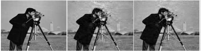
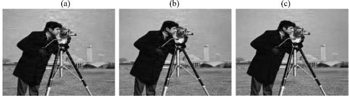
Table 1. PSNR Performance and Running time comparison of several techniques

Sampling rate M/N		0.5		0.6		0.7		0.8
		PSNR	TIME	PSNR	TIME	PSNR	TIME	PSNR	TIME
Lena	SP	25.76	52.38	26.49	58.20	26.90	74.92	27.17	77.39
	OMP	26.56	5.65	30.06	5.83	31.38	5.97	32.26	6.11
	ROMP	21.84	1.51	25.59	2.20	27.36	2.27	29.26	2.46
	GOMP	28.82	4.66	31.13	7.50	33.39	11.34	35.89	15.35
	GOAMP	26.82	8.73	29.18	9.81	31.51	9.89	36.42	11.54
	Proposed Method	31.58	4.51	33.13	5.01	34.09	5.63	35.89	6.82
Peppers	SP	24.03	57.19	24.54	64.35	24.97	72.33	25.18	73.26
	OMP	25.80	8.77	26.75	6.78	27.58	6.61	28.52	6.80
	ROMP	21.03	2.38	22.05	2.25	25.44	2.41	29.69	2.73
	GOMP	27.50	5.20	29.55	8.51	31.60	11.35	34.00	15.26
	GOAMP	27.27	8.98	30.15	12.32	29.84	10.40	32.6	12.83
	Proposed Method	29.50	3.45	32.05	6.60	33.44	6.35	34.04	5.86

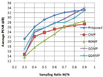
Fig.2. Comparison of Average PSNR (dB) for varying Sampling ratios M/N

• B.    Reconstruction Error and Running Time

For the noise less case, the performance of the algorithm can be seen in terms of the reconstruction error and running time. The proposed method uses N- dimensional image with M=128 measurements and ^max is in the range {10, 45} and a=10,P =7 . For the individual sampling ratio, reconstruction simulations are done on 20 standard grayscale .bmp images. The reconstruction error is given in the form of Average Normalized Mean-Squared-Error (ANMSE), which is defined as:

ANMSE _{= ∑} 20  ^1-1

‖ x- ̌‖

‖ X_{t ‖}

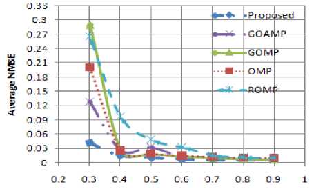
where xt is the itℎ original image and ̌i is the recovered form of it. The exact recovery condition is represented in terms of:‖x - ̌‖2≤10 2‖X‖2 . The reconstruction rate remains acceptable with minimal ANMSE for the proposed algorithm. The Fig. 3 depicts ANMSE for different Gaussian measurements. The ANMSE for the proposed method remains minimal for a=10,p=7. The recovery performance is better as the given algorithm offers lesser Average Normalized MSE with the different sampling ratios. Hence, it offers higher recovery percentage than the compared methods for the given dataset of images. But, for the run times, increment in a,P slows down the algorithm. It is because of the decrease in the increment of the size of the support set per iteration through the algorithm. In Fig. 4, the average running time for the different recovery algorithms is compared. The running time elapsed for ROMP algorithm is the minimum but simultaneously the visual quality and recovery performance is poor. The implemented method has acceptable running time, comparable to ROMP at M/N=0.3, 0.4, 0.5. Though, the running time increases with increment in sampling ratio but still less than OMP, SP and others existing recovery methods. Thus, the proposed method is capable of recovering the sparse images with better quality within acceptable running time.

Sampling Ratio M/N

Fig.3. Average normalized Mean-squared Error (ANMSE) comparison for varying Sampling ratios M/N

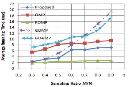
Fig.4. Comparison of Average Running Time (sec) for varying Sampling ratios M/N

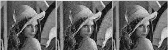
• C.    Reconstruction Results for Noisy Observations

As the signal transmission system channel may add a lot of noise that may lead to the distortion of information. It is required to study the recovery performance of the given algorithm in the presence of noise. In this paper, white Gaussian noise is added with the specified value of signal to noise ratio (SNR) =10, 15, 20, 25. The reconstruction result for the proposed method with added noise is depicted in Fig. 5. The Fig. 5 shows that the algorithm provides effective recovery for the twodimensional images but the quality goes lower for lower sampling ratio. The simulation results of PSNR and running time for different value of SNR is provided by Table 2. A comparative analysis for the image reconstruction is given in Table 3 with different SNR and sampling ratio M/N= {0.5. 0.6, 0.7, 0.8}. The comparison conveys that the recovery performance of the given method is better than the other algorithms, which are not able to recover accurately. The proposed method outworks the other method in terms of PSNR for reconstruction in the presence of noise.

(a)                         (b)                         (c)

(d)                             (e)                         (f)

Fig.5. Reconstruction result of proposed method for noisy observations. For M/N=0.5, (a) SNR=10 (b) SNR=15 (c) SNR=20. For M/N=0.8 (d) SNR=10 (e) SNR=15 (f) SNR=20.

• D.    Performance Analysis of algorithms

In order to evaluate the performance of the given algorithm, the effect of recovery performance for different algorithms is demonstrated. The comparative analysis of the recovery performance of the different algorithms relative to the proposed method is given in Fig 6. It shows that the proposed method is capable of recovering the fine and near the edge details as comparison to the reconstructed image by the other methods. The proposed method can take into account the effect of noise added while recovering the sparse image and is able to provide practical reconstruction. A careful comparative analysis of the proposed method with that of the existing methods in the presence of noise demonstrates higher value of PSNR within reasonable time period. Similarly, in the case of added Gaussian noise, quality of recovered image for each of the tabulated algorithm is shown in Fig. 7. It shows that for lower value of SNR, for example SNR=5 dB, the recovery accuracy is ineffective as comparison to the noiseless situations. The output PSNR value is low but as the value of SNR increases, the value of PSNR increases with better recovery performance. It depicts that even in the presence of noise; the proposed method is capable of reconstructing the image precisely. Though, there is only minor difference in the visual outcome of GOAMP algorithm relative to the proposed method. However, the details of the fine region are recovered accurately with proposed method. The reconstruction results depicts that the given method works efficiently and perform more accurate for faster reconstruction of the image and is much more sophisticated than the older method SP, OMP, CoSaMP and GOMP. On the contrary, the reconstruction probability of the proposed method decreases with factor n. And, it provides better results with n E [1,4]. Hence, suitable value of n is required and the backward step P < a — 1 for the accurate recovery of the sparse image.

Table 2. Comparison of PSNR and running time when SNR=10,15,20,25,30

SNR	10		15		20		25		30
Sampling Ratio M/N	PSNR	Time	PSNR	Time	PSN R	Time	PSNR	Time	PSNR	Time
0.5	20.86	4.30	25.07	4.35	28.30	4.19	29.89	4.20	30.90	4.31
0.6	21.52	4.60	26.10	4.62	29.67	4.73	31.79	6.39	32.50	6.64
0.7	22.00	4.88	26.70	4.99	30.68	4.97	32.95	9.29	33.73	9.40
0.8	22.35	4.97	27.13	5.47	31.07	4.92	33.76	15.07	34.51	12.52

Table 3. Performance analysis for noisy observations when M/N=0.5

SNR	5		10		15		20
Reconstruction algorithms	PSNR	Time	PSNR	Time	PSNR	Time	PSNR	Time
SP	12.89	53.79	17.14	56.75	20.83	57.85	20.83	40.38
OMP	10.19	17.603	14.79	13.10	19.11	10.46	20.43	8.0
ROMP	15.11	1.77	17.21	1.95	19.32	1.93	20.03	2.16
GOMP	12.21	5.45	16.78	4.27	20.85	4.70	24.31	4.71
GOAMP	11.66	9.06	15.61	8.42	20.44	8.15	24.16	8.15
Proposed Method	16.19	8.39	20.64	4.41	25.07	4.35	28.30	4.19

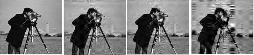
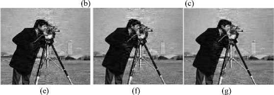
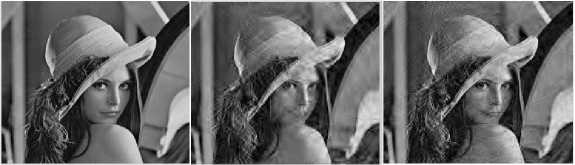
Fig.6. Comparison of reconstruction results for M/N=0.5 (a) Original image (b) SP method (c) OMP method (d) ROMP method (e)GOMP method (f) GOAMP method (g) Proposed method.

(d)                          (e)                           (f)

Fig.7. Comparative demonstration of the reconstruction result for sampling ratio M/N=0.5 and SNR=30 dB (a) Original image (b) Image reconstructed with SP (c) Image reconstructed with OMP (d) Image reconstructed with ROMP (e) Image reconstructed with GOMP (f) Image reconstructed with GOAMP .

• VI. Conclusion

This paper proposes an algorithm for forwardbackward movement in adaptive Generalized OMP under certain stopping conditions for CS based image recovery. The stopping conditions are refined by cumulative coherence and the method works on low frequency components for saving the memory storage. This two-stage technique expands the support set by forward step with the size of indices a and then the selected indices of the support estimate is cropped by the backward step with a step size of p . Additionally, the size of the forward and backward step increases adaptively for reduction in residue through the algorithm. As compared to existing techniques, this method provides the advantage of removing the misidentified or non-significant elements with backward step. The step size also increases adaptively and the algorithm is terminated with the stopping condition. Simulation results show that the given method improves reconstruction for Gaussian measurement both in noiseless and noisy cases. Hence, it recovers images accurately with significant PSNR. Even at lesser number of observations, such as at M =0.3, 0.4, 0.5, the proposed method provides the better results i.e. the reconstruction result is clearly visible at lesser observations. However, for the sampling ratios equal to or greater than 0.9, the results become comparable with Generalized OMP. But, when the magnitude of nonzero elements is not comparable, proposed method provides better performance. Consequently, it is concluded that proposed method is capable of providing better recovery performance for image recovery from compressed observations in both noisy and noise-less cases.