Compromise Hypersphere for Multi-Criteria Dynamic Programming

Published Online January 2015 in MECS DOI: 10.5815/ijieeb.2015.01.01

The paper presents a usage of compromise hypersphere in multi-criteria dynamic programming. The form of dynamic programming model is taken from the works by Sitarz [1] and [2]. The most recent contributions to dynamic programming in the view of the proposed approach are as follows. Bazgan et al. [3] present the approach of ordered structures in dynamic programming. Sitarz [4] shows a usage of dynamic programming into multiple knapsack problem. In [5] the stochastic dynamic programming on compact state spaces is discussed. Whereas the idea of compromise hypersphere comes from the work by Gass and Roy [6]. The source of the compromise hypersphere is the compromise programming presented in [7] and [8]. By using the presented method, we obtain the decision analysis tool in multi-criteria dynamic problems. The method consists of three steps. In step 1 we determine a set of efficient realizations in discrete dynamic programming model by using the forward algorithm. In step 2 we find the compromise hypersphere, which means a kind of compromise between the values of efficient realizations. In step 3 we build the ranking of efficient realization by using the compromise hypersphere. Moreover, by using the presented method we are able to take into account the risk aversion of the decision maker by choosing the parameter of the method. The general form of the presented model allows us to use it in many problems, particularly we apply the method in the market model.

The paper consists of the following sections. Section II presents discrete dynamic programming model with forward algorithm for finding the efficient realizations. Section III introduces compromise hypersphere method with the proposition of risk aversion measure. Section IV shows an application of the proposed method in the market model. The paper is summarized in the final section V.

• II.    Dynamic Decision Process

Discrete dynamic process is considered. The notation of this process is described in Table 1.

• A.    Period criteria functions

Let P stand for the process. The period criteria function in the period t (t=1, … T) is the function:

f t :R t → ℝ ^k                    (1)

where ℝ ⁿ denotes the n-dimensional vector of real numbers. Next, we assume the following simplification of the notation:

f t ( s t , s t+1 ) = f t ( (s t , s t+1 ) )                  (2)

Below, we present the definitions of the multi-period criteria function by using the binary operator °, which links the period valeus.

• -    Partial backward criteria function F t^← :R t^← (S t ) → ℝ ^k :

Ft' = ft ° (ft-1 ° C- (fj-1 ° fr) -))(3)

• -    Partial forward criteria function F t^→ :R t^→ (S t ) → ℝ ^k :

Ft" = ((^(fi ° f2 ) ...) ° f-2 ) ° ft-1

• -    Multi-period criteria function F:R → ℝ ^k :

F = ((^(fi ° f2 ) ° ...) ° fr-1) ° fr

Table 1. Notation of dynamic process.

Symbol	Meaning	Elements description
T	The number of stages	t ∈ {1, … ,T}
S t	The set of feasible states at the beginning of the stage t	S t
D t (s t )	The set of feasible decisions at the beginning of the stage t, in the state s t	d t (s t )
R	Realizations of the processsequence of the succeeding states	r=(s 1 ,s 2 ,.., s T, ,s T+1 )
R t	The set of stage realizations at the beginning of the stage t	r t = (s t , s t+1 )
R t ← (s t )	The set of partial realizations of the process beginning at the point t and the state s t	r t ← (s t ) =(s t , … ,s T+1 )
R t → (s t )	The set of partial realizations of the process ending at the point t in the state s t	r t → (s t ) = (s 1 , … , s t )
R t ← (S t )	The set of partial realizations beginning at the point t	r t ← (s t ): s t ∈ S t
R t → (S t )	The set of partial realizations ending at the point t	r t ← (s t ):  s t ∈ S t
P	The process in which T, S t , D t (s t ) were defined

Next, we assume the notation

Ft←(Rt←(St)) = {Ft←(Rt←(st)): st∈St}(6)

Ft→(Rt←(St)) = {Ft→(Rt→(st)): st∈St}(7)

F(R) = {F(r): r∈R}(8)

• B.    Efficient realizations

Non-dominated vectors of the set A ⊂ ℝ ^k denoted as ND(A) are described in the following way:

ND(A) ={a∈A: ∀x∈A a≤x ⇒ x=a}(9)

The realization r ∈ R is called the efficient realization when

F(r) ∈ ND {F(R)}(10)

The set of all efficient realizations is denoted as EFF(R).

• C.    Forward Algorithm

The above terms launch a problem of finding all efficient realizations. The detailed description of the methods used for such problems may be found in the work by Trzaskalik and Sitarz [9]. Moreover, the work by Sitarz [10] presents the heuristic methods for such problems. Below, we present the forward algorithm from the work of Sitarz [11]:

Step 1. Find

ND{f₁(R₂ ^→ (s₂)}, for all states s₂ ∈ S₂.

Step 2. Find

ND{F₂ ^→ (R₃ ^→ (s₃)}, for all states s₃ ∈ S₃.

using the values found in step 1

ND{F 2^ (R 3^ (s 3 )} = ND{f 2 (s 2 , S 3 )”ND(f 1 (R 2^ (s 2 )) ):

s 3 ∈ D 2 (s 2 )}                                          (11)

Step t , for t=3, … , T . Analogically to step 2, find

ND {F_t ^→ (R_t+1 ^→ (s_t+1)}, for all states s_t+1 ∈ S_t+1.

Step T+1. Find max {F(R)}

ND {F(R)}=ND{ND F T+1^→ (r t+1^→ (s T+1 )):s T+1 ∈ S T+1 }   (12)

At the same time, we get efficient realizations EFF(R) which relate to the found maximal values.

• III.    Compromise Hypersphere Method

The aim of the method is to rank the efficient realizations in discrete dynamic programming model. The main idea of the proposed method comes from the work by Gass and Roy [6]. The method consists of three steps. Step 1 presents an initial problem of decision making - finding a set of efficient realziations. In step 2 we look for a hypersphere which we call a compromise hypersphere. In this case the word compromise means a surface of compromise over the values of nondominated extreme solutions. Thus, we look for the points which are closest to this surface. It means that the point closest to this surface is the best compromise solution. In step 3 we built ranking of points by using distance to the compromise hypersphere. In detail, the method looks as follows:

Step 1. Determine a set of efficient realizations in discrete dynamic programming model by using the forward algorithm presented in subsection II.C. We will denote these efficient realizations as: r ¹ , r ², . ., r n .

г lr (a, b) = H

Step 2. Find a hypersphere with the centre y0e Kk and radius r0e К by solving the program min iq ( [r0,...,r], [12(F(r1),y0),...,lk(F(rn),y0)] )   (13)

y , r ₀

where q e[1, to] is parameter ln is function belonging to the family of metrics

Vs : К ^s x K ^s ^ K with the following form:

s

S a - - b\ , ^{r G [1,} * )               (14)

i = 1

max | a, - b |, r = to

We will denote the optimal solution of (13) as y0q , q r and the minimal value of the cost function as min(13)q . Moreover, wherever it does not cause notion misunderstanding, we will omit index q i.e. y0 , r and min(13) .

Step 3. Find the ranking of the points r ¹ , r ² , …, r ⁿ based on the distance from the previously found hypersphere in step 2, using values

|r - 12 (F(r ' ), y ⁰)|                      ⁽¹⁵⁾

We will particularly look for the point r ⁱ closest to the hypersphere:

min | r ₀ - l k (F(r¹), y ⁰ )|              ⁽¹⁶⁾

We will denote the opti m al solution of (16) as i , the optimal extreme poi nt as r ⁱ , and the minimal value of the cost function as min(16) .

• A. Risk aversion measure – the choice of q

The choice of the metric (the value of q ) should go along with some preferences of the decision maker, which is described by Ballestero [12] who concludes his works by sentence: “The greater risk aversion the greater q -metric to use. Metric q = to corresponds to extremely high risk aversion”. Thus the preferences of the decision maker can be incorporated in the presented method by choosing the parameter q – representation of the risk aversion.

By using the above theory, we can formulate the following comments to setting parameter q :

• -    q =1 corresponds to extremely low risk aversion,

• -   q = to corresponds to extremely high risk aversion,

• -    q e (1, to ) corresponds to risk aversion between low and high.

The above scale, [1, to ], can be hard to use in practice. Thus, we propose to transform interval [1, to ] to interval [0, 1] by a given bijection f , for example by f ( q )=

(2/ л )• arctan ( q - 1). After using such a transformation f the decision maker gives a value from interval [0,1] to describe his risk aversion in the following way:

• -   f ( q )=0 corresponds to extremely low risk aversion,

• -   f ( q )=1 corresponds to extremely high risk aversion,

• -   f ( q ) e (0, 1) corresponds to risk aversion between

low and high.

• IV.    Application in the market model

The form of the problem is inspired by the work of Ekeland [13]. We should add that the problem assumes indivisibility of goods available on the market, whereas in the mentioned work, the value of the goods is described by any nonnegative real number.

The presented problem refers to the theory of demand that describes the economic market, in which there is a group of participants (hereafter referred to as consumers). You can purchase a certain amount of goods on the market. Generally, the consumers aim to reach the greatest satisfaction from the purchase of goods. The satisfaction is described with the help of the utility function value. The aim of the problem below is to find such a distribution of goods among the consumers. Below, we present the detailed description of the problem.

n – the number of goods on the market. Particular goods will be denoted by the letter i, that is i e {1, . ,n}. We assume that the goods are indivisible which means that each commodity appears in a value belonging to the set N= {0, 1, 2, . }.

m – the number of consumers. Particular consumers will be denoted by the letter k, that is k e {1, _ ,m}.

Qi - value of ith commodity available on the market, Qi e N, for ie {1,.,n}.

Q = ( Q 1 , ..., Q _n) - joint value of goods available on the market.

u_k: N ⁿ ^ K - utility function of k th consumer (describes the preferences of k ^th consumer depending on the value of the possessed goods).

Feasible allocations are the vectors x=(X11, ., xn1,.....X1k, ^, xnk,.. X1m, ^, xnm)eNnxm (17)

which satisfy the condition:

m

V ie{i,.,n}    S x ik = ^Q i             (18)

k=1

Feasible allocations describe the ways of distribution of goods among the consumers and they will be written down also as (x i^k : i=1,.., n; k=1,...,m).

The components x 1^k , ., x_n ^k denote values of proper goods which are assigned to the k ^th consumer. For example, x 2⁵ means the number of the second commodity assigned to the fifth consumer.

A - the set of all feasible allocations.

Each feasible allocation x=(x 11 , ., x n¹ , ..., x 1^k , .. x nk,..... x 1^m , ., x_n ^m ) is connected with the vector u(x):

u(x) = (U1(X11, ., Xn1),., Um(X1m, ., Xnm))(19)

Vector u(x) gives the values of the utility function of all consumers.

Pareto Optimal allocations are the vectors y=(y11, . yn1,....., y1m, ., ynm) eA(20)

which satisfy the following condition:

u(y) ∈ ND {u(x): x∈A}(21)

• A.    Numerical example

The following numerical example is taken from work by Sitarz [1]. We consider a model with the following data:

• •    there are 3 consumers on the market, i.e. m=3,

• •    there are 3 commodities to distribute, i.e. n=3,

• •    there are 2 of each commodity, i.e. Q 1 = Q 2 = Q ₃=2.

The utility functions of the particular consumers have the form:

• •   U i (X i , X 2 , X 3 ) = X 1 + 2X 2 + 3x 3

• •   U 2 (X i , X 2 , X 3 ) = X 1 - X 2 - X 3

• •   U 3 (X i , X 2 , X 3 ) = 3X 1 + X 2 + X 3

• B.    Construction of the process

We have 6 periods:

T = n ⋅ (m-1) = 3 ⋅ 2=6

Feasible states

S 1 =s,

We find the remaining feasible states by using the formula:

S t = {0, 1,..., Ω ⌊ (t-2):(m-1) ⌋ +1 }.

Thus

S 2 = S 3 = Ω 1 = 2.

S 4 = S 5 = Ω 2 = 2.

S₆ = S₇ = Ω ₃ = 2.

Feasible decisions for t∈ {1, 3, 5} and st∈St

D t (s t ) = S t+1 = {0, 1, 2}.

for t ∈ {2, 4, 6}

D t (0) = {0}, D t (0) = {0, 1}, D t (0) = {0, 1, 2}

• C.    Values of the period criteria function

• •    Case I, for t e {2, 4, 6}

Table 2 shows the values of the stage criteria functions in this case.

• •    Case II, for t e {1, 3, 5}

Table 3 shows the values of the stage criteria function in this case.

The graph of the described multi-period decision process is shown in figure 1, we have given only the chosen values of the criteria function, whereas we have given all feasible states and decisions

• D.    Pareto-optimal allocations

Now, we will generate Pareto Optimal allocations. We will find them by solving the DP problem (figure 2). We will use the algorithm from subsection II.C. The calculations are illustrated in table 4. Simultaneously, together with the values obtained in the last row of table 4, we obtain 16 Pareto Optimal allocations. Below, all maximal values of the utility function, together with the relevant allocations are presented in table 5.

• E.    Compromise hypersphere method

We will conduct the method described in section III.

Step 1. Pareto Optimal allocations mean the efficient realizations of the considered dynamic process. Thus, the efficient realizations (obtained earlier in subsection 4.3) have the following notation: r ¹ , r ² , .., r ¹⁶ .

Step 2. Decision maker chooses the parameter q as the representation of his risk aversion following the rule: The greater risk aversion the greater q . In this case we consider q =2.

The optimal values of the objective function of the problem (13) are as follows:

min(13)2= 0.473            (22)

Step 3. On the basis of the distance to the previously found hypersphere we obtain ranking presented in table 6.

Table 2. Values of the period criteria function w for t ∈ {2, 4, 6}.

f t (s t , s t+1 )		t
		2	4	6
(s t , s t+1 )	(2,2)	(0,0,6)	(0,0,2)	(0,0,2)
	(2,1)	(0,1,3)	(0,1,1)	(0,1,1)
	(2,0)	(0,2,0)	(0,2,0)	(0,2,0)
	(1,1)	(0,0,3)	(0,0,1)	(0,0,1)
	(1,0)	(0,1,0)	(0,1,0)	(0,1,0)
	(0,0)	(0,0,0)	(0,0,0)	(0,0,0)

Table 3. Values of the period criteria function w for t ∈ {1, 3, 5}.

f t (s t , s t+1 )		t
		1	3	5
(s t , s t+1 )	(s,2)	(0,1,0)	-	-
	(s,1)	(1,1,0)	-	-
	(s,0)	(2,1,0)	-	-
	(2,2)	-	(0,1,0)	(0,1,0)
	(2,1)	-	(2,1,0)	(3,1,0)
	(2,0)	-	(4,1,0)	(6,1,0)
	(1,2)	-	(0,1,0)	(0,1,0)
	(1,1)	-	(2,1,0)	(3,1,0)
	(1,0)	-	(4,1,0)	(6,1,0)
	(0,2)	-	(0,1,0)	(0,1,0)
	(0,1)	-	(2,1,0)	(3,1,0)
	(0,0)	-	(4,1,0)	(6,1,0)

Table 4. Calculations obtained with the help of the algorithm from subsection 2.3.

t	ND{F t → (R t → (0)}		ND{F t → (R t → (1)}	ND{F t → (R t → (2)}
1	(2,1,0)		(1,1,0)	(0,1,0)
2	(2,0,0), (1,1,0), (0,2,0)		(1,0,3), (0,1,3)	(0,0,6)
3	(6,0,0), (5,1,0), (4,2,0), (5,0,3), (4,1,3), (4,0,6)		(4,0,0), (3,1,0), (2,2,0), (3,0,3), (2,1,3), (2,0,6)	(2,0,0), (1,1,0), (0,2,0) , (1,0,3), (0,1,3), (0,0,6)
4	(6,0,0), (5,0,3), (4,0,6), (3,1,0), (2,2,0) (2,1,3), (1,2,0), (0,4,0) (0,2,3)		(4,0,1), (3,0,4), (2,0,7) (1,1,1), (0,2,1) (0,1,4),	(2,0,2), (1,0,5), (0,1,5), (0,0,8)
5	(12,0,0), (11,0,3), (10,0,6), (9,1,0), (8,2,0) (8,1,3), (7,2,0), (6,4,0) (6,2,3), (8,0,7), (6,1,5), (6,0,8)		(9,0,0), (8,0,3), (7,0,6), (6,1,0), (5,2,0), (5,1,3), (4,2,0), (3,4,0), (3,2,3), (5,0,7) (3,1,5), (3,0,8)	(6,0,0), (5,0,3),(4,0,6), (3,1,0), (2,2,0) (2,1,3), (1,2,0), (0,4,0) , (0,2,3), (2,0,7), (0,1,5), (0,0,8)
6	(12,0,0), (11,0,3), (10,0,6), (8,0,7), (6,0,8), (6,1, 0), (5,2,0) (5,1,3), (3,4,0) (3,2,3), (3,1,5), (0,8,0), (0,4,3), (0,0,8), (0,2,4),		(9,0,1), (8,0,4), (7,0,7) (5,0,8), (3,0,9)	(6,0,2), (5,0,5), (4,0,8) (2,0,9), (0,0,10)
ND F(R)		(12,0,0), (11,0,3), (10,0,6), (8,0,7), (6,0,8), (6,1, 0), (5,2,0), (5,1,3), (3,4,0) (3,2,3), (3,1,5), (0,8,0) (0,4,3), (0,2,4),(3,0,9), (0,0,10)

Table 5. Values of the utility function, together with the relevant Pareto Optimal allocations.

(u 1 , u 2 , u 3 )	Pareto optimal allocation
(12, 0 ,0 )	r1 =(2,2,2, 0,0,0, 0,0,0)
(11, 0, 3)	r2= (1,2,2, 0,0,0, 1,0,0)
(10, 0, 6)	r3= (0,2,2, 0,0,0, 2,0,0)
(8, 0, 7)	r4= (0,1,2, 0,0,0, 2,1,0)
(6, 0, 8)	r5= (0,0,2, 0,0,0, 2,2,0)
(6, 1, 0)	r6= (1,1,1, 1,1,1, 0,0,0)
(5, 2, 0)	r7= (0,1,1, 2,1,1, 0,0,0)
(5, 1, 3)	r8= (0,1,1, 1,1,1, 1,0,0)

(u 1 , u 2 , u 3 )	Pareto optimal allocation
(3, 4, 0)	r9= (0,0,1, 2,2,1, 0,0,0)
(3, 2, 3)	r10= (0,0,1, 1,2,1, 1,0,0)
(3, 1, 5)	r11= (0,1,1, 1,1,1, 1,0,0)
(0, 8, 0)	r12= (0,0,0, 2,2,2, 0,0,0)
(0, 4, 3)	r13= (0,0,0, 1,1,2, 1,0,0)
(0, 2, 4)	r14= (0,0,0, 1,1,2, 1,1,0)
(3, 0, 9)	r15= (0,0,1, 0,0,0, 2,2,1)
(0, 0, 10)	r16= (0,2,2, 0,0,0, 2,2,2)

Table 6: Ranking obtained by using compromise hypersphere method

1. r7	9. r5
2. r2	10. r10
3. r11	11. r16
4. r13	12. r6
5. r1	13. r15
6. r3	14. r9
7. r8	15. r4
8. r14	16. r12

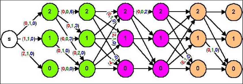
Fig. 1. The graph of the decision process with chosen values of period criteria functions.

• V.    Summary

We considered a multi-criteria dynamic process with a finite number of periods, states and decision variables. To obtain the efficient realizations, we used the forward algorithm presented in subsection II.C. Next step was to rank the obtained efficient realizations, which was made by using the compromise hypersphere method described in section III. Such general approach allowed us to apply the presented model to many multi-period, multi-criteria decision making problems. The exemplary area of applications of the presented dynamic model was the market model described by Elkeland [8]. We used the market model to illustrate the application of the presented theory. Further research and problems to solve are as follows:

• -    Using other structures to describe the preferences of decision maker: interval coefficients, fuzzy numbers or stochastic orders,

• -    Introducing interactive version of the compromise hypersphere method,

• -    Comparison with other methods based on compromise programming, for example with methods from work by Opricovic and Tzeng [14].

• -    Applying the sensitivity analysis of the obtained ranking, [15].

Acknowledgment

This project was financed with means of the National Science Centre (Poland) according to decision number DEC-2013/11/B/HS4/01471.