Computational Intelligence in Magnetic Resonance Imaging of the Human Brain: The Classic-Curvature and the Intensity-Curvature Functional in a Tumor Case Study

Published Online April 2014 in MECS

Since the inception of signal-image interpolation through the works of Isaac Newton [1], an enormous amount of studies corroborated with formulations of improved interpolation paradigms have been reported in the literature. The most representative studies [2-4] have guided the discovery of the unifying framework [5] and the unified framework [6] for the improvement of the interpolation error. From the two frameworks [5, 6], two mathematical engineering tools have been conceived.

The two mathematical engineering tools are: (i) the Classic-Curvature [6] and (ii) the Intensity-Curvature Functional [5-8]. The methodological characteristics for the calculation of the two aforementioned mathematical engineering tools are the same regardless of the model polynomial function fitted to the signal-image data. The only requirement is that the model polynomial function benefits of the property of second-order differentiability in its interval of definition, which is that property that makes the model polynomial function to have non null and continuous second-order derivatives. The key to the formulation of the mathematical engineering tools presented here is thus the computational intelligence of the Classic-Curvature, which is calculated summing up all of the second-order derivatives of Hessian of the model polynomial function fitted to the signal-image data. The calculation of the Classic-Curvature is also beneficial to the calculation of the Intensity-Curvature Functional, which is defined through the ratio between two terms, both of them inclusive of the intensity-curvature content of the signal-image. The two terms are: (i) the integral of the product between the Classic-Curvature and the value of the signal-image intensity, both of them calculated at the grid node, and (ii) the integral of the product between the Classic-Curvature and the value of the signal-image intensity, both of them calculated at the intra-pixel coordinate used to re-sample the signal. Thus, resampling, which is inherent to interpolation, is also another piece of computational intelligence, which allows the calculation of both of the Classic-Curvature and the Intensity-Curvature Functional. Specifically, the intrapixel coordinate chosen to calculate the aforementioned mathematical engineering tools is such to determine the information content of the resulting images and thus, in the present research, it is relevant to the information extracted from the Magnetic Resonance Images.

In this paper, emphasis is given to two model polynomial functions, namely: the bivariate and the trivariate cubic Lagrange polynomials [6, 8]. It is here shown that from the aforementioned two model polynomial functions it is possible to calculate the Classic-Curvature and the Intensity-Curvature Functional, which extract information from the original MRI images. Therefore, through the use of the Classic-Curvature and the Intensity-Curvature Functional of the model polynomial functions it is possible to highlight characteristics of the signal-image which are seen in the MRI domain. In the theory section, the procedure for the calculation of the mathematical engineering tools will be presented. The results section will present images obtained fitting both of the bivariate and the trivariate cubic Lagrange polynomials to pathological MRI data of the human brain showing a tumor. The results section will focus on the capability of the Classic-Curvature and the Intensity-Curvature Functional to perform feature extraction from the original image, showing that it is possible to add complementary information to the original MRI. In the discussion and conclusion sections the practical implications of this research will be presented placing the emphasis on the methodological approach and also on the value added to the original MRI through the use of the two mathematical engineering tools used in this piece of research.

• II.    Theory

Let the bivariate and trivariate cubic Lagrange polynomials g( x ) = g(x₁, x₂…x_n) be defined as:

of all second order derivatives of the polynomial with respect to all of the variables and all the covariates.

n

® ( x ) = Z

1 = k = 1

^{: x :}

^S x i d x k

In (4) 'n' defines the dimensionality of the polynomial. Let the intensity-curvature term before interpolation E 0 ( x ) [5], and the intensity-curvature term after interpolation E IN ( x ) [5] be defined as per (5) and (6).

xx

The definition of the Intensity-Curvature Functional is:

g( x ) = f( 0 ) + a 2 • a

3ni

Z h i Z X k 1 = 0 ^ k = 1 J

+ а з • a

2ni

Z m i Z X k i = 0 ^ k = 1 J

The constant f( 0 ) is the pixel (2D) or the voxel (3D) intensity. The constant 'a' is the parameter of the cubic Lagrange polynomial and is here named as the constant parameter in (1). In (1), 'h_i' and 'm_i' are the coefficients of the polynomial, 'n' defines the dimensionality of the polynomial and 'i' is the exponent of each of the sums of the independent variables. Positions (2) and (3) hold true, with 's' and 'r' defining how many pixels are included into the polynomial convolutions.

« 2 = £f(p)                     (2)

p = 1

а з = Z^ P)                    (3)

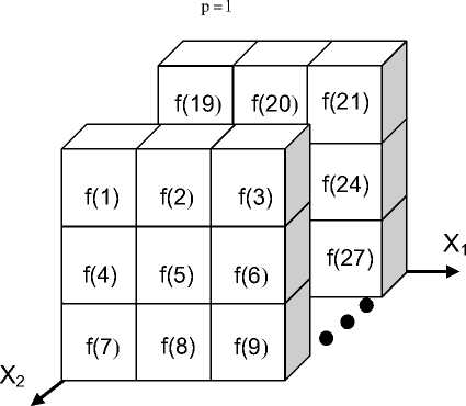
Fig. 1. The layout of the pixels in the neighborhood of the bivariate and trivariate Lagrange (g( x )) model polynomial functions.

Therefore, the Classic-Curvature of the bivariate cubic

Lagrange polynomial (1) is given in (4) and it is the sum

AE( x ) =

E o ( x ) Ein( x )

It is possible to calculate ΔΕ( x ) of both of the bivariate and the trivariate cubic Lagrange polynomials through (7) [6].

III. RESULTS

This section presents results obtained with Magnetic Resonance images of the human brain when the bivariate cubic Lagrange polynomial was fitted to the signal-image data. Also, the MRI volumes inclusive of the slices shown in this section were processed with the trivariate cubic Lagrange polynomial fitting the math model as shown in the neighborhood of Fig. 1, and the results are shown in the following figures. The images which were obtained fitting to the 2D signal-data the bivariate cubic Lagrange polynomial were re-sampled of 0.1mm along the x direction and 0.1mm along the y direction. The images which were obtained fitting to the 3D data the trivariate cubic Lagrange polynomial were re-sampled of 0.1mm along the x direction and 0.1mm along the y direction and 0.1mm along the z direction.

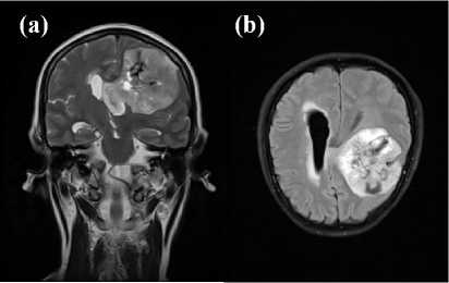
Fig. 2. Magnetic Resonance Imaging showing the tumor: (a) the image is made of a 262 x 320 pixels matrix with pixel size of 0.78mm x 0.78mm; (b) the image is made of a 260 x 320 pixels matrix with pixel size of 0.78mm x 0.78mm. The images were cropped to the regions of interest.

Fig. 2 shows two of the MRI images employed in this piece of research, which are referred here as to be the original MRI. The tumor is visible in the human brain in both of the pictures shown in Fig. 2.

Fig. 3 shows the couple of images: Classic-Curvature in (a), obtained with the bivariate cubic Lagrange polynomial and the Intensity-Curvature Functional in (b), obtained with the trivariate cubic Lagrange polynomial. Specifically, since it is the object of this piece of research to assess the capability of the two mathematical engineering tools to provide complementary information through feature extraction from the original MRI, the emphasis is in the comparison of the appearance of the Classic-Curvature and the Intensity-Curvature Functional images shown in Fig. 3 and Fig. 4 with the original MRI shown in Fig. 2.

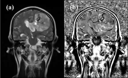
Fig. 3. In reference to the image shown in Fig. 2a, (a) shows the ClassicCurvature image and (b) shows the Intensity-Curvature Functional image. In (a) is visible the reproduction of all of the human brain features. In (b) it can be seen the tumor inside the thin line that surrounds the pathology.

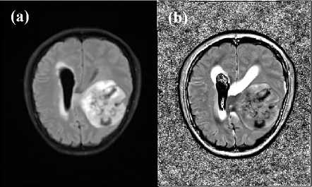
Fig. 4. In reference to the image shown in Fig. 2b, (a) shows the Classic-Curvature image and (b) shows the Intensity-Curvature Functional image. The Intensity-Curvature Functional shows a thin line which encapsulates the tumor and this more evident in (b) than in (a). The thin line is lateral to the tumor. Also, the pixels of the IntensityCurvature Functional were calculated with the trivariate cubic Lagrange polynomial, which process the MRI data using pixels placed in three consecutive slices, and so the ventricle is seen in (b).

The value of the constant parameter in (1) was set to the value of 2.54 in both of Fig. 3 and Fig. 4. While Fig. 3a (Classic-Curvature image) reproduces faithfully the features of the image seen in Fig. 2a, the IntensityCurvature Functional of Fig. 3b shows the demarcations of the brain structures, the distinction between gray and white matter and also the tumor. Also, visible in Fig. 3b more than in Fig. 3a is the contour line enclosing the tumor.

Fig. 4 shows the Classic-Curvature image in (a) obtained when fitting the bivariate cubic Lagrange polynomial, and the Intensity-Curvature Functional image in (b) obtained when fitting the trivariate cubic Lagrange polynomial to the human brain data. The images in Fig. 3 and Fig. 4 show the tumor with a neat distinction between the Classic-Curvature image, which is similar to the original MRI, and the Intensity-Curvature Functional image which focuses on the contours of the tumor and the visualization of the pressure exercised by the tumor on the ventricles of the human brain.

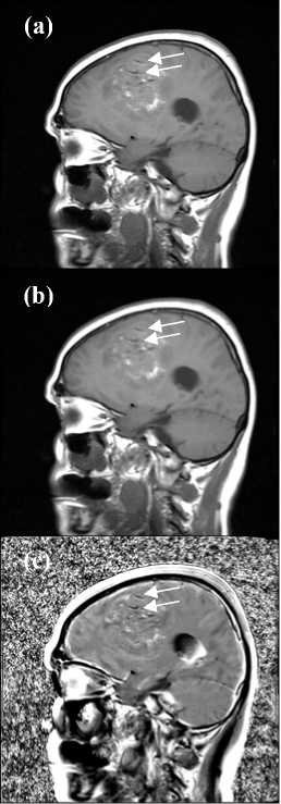
Fig. 5. The Magnetic Resonance Imaging showing the tumor is (a). The image is made of a 512 x 512 pixels matrix with pixel size of 0.45mm x 0.45mm. The Classic-Curvature image and the Intensity-Curvature Functional image are presented in (b) and in (c) respectively. The contrast is enhanced in all of the pictures, and when comparing (a) with (b) and (c), some presumed blood vessels are highlighted (see white arrows).

Fig. 5 shows in (a) the original MRI with the tumor distinguishable through the white nuances. Fig. 5b and Fig. 5c show the Classic-Curvature image and the Intensity-Curvature Functional image, respectively, which were obtained from the original MRI shown in (a). The white nuances are repeated in the Classic-Curvature image of Fig. 5b, and the nuances are seen also in the Intensity-Curvature Functional image of Fig. 5c.

A remarkable difference between Fig. 5b and Fig. 5c is that, while the former shows a flat image which is very much alike the one seen in Fig. 5a, the latter elicits the perception of the depths of both the anatomical structures of the brain and the tumor. As indicated by the two white arrows in Fig. 5c, the Intensity-Curvature Functional image is also capable of marking the presumed vessels of the human brain, and so, such brain vessels, which are observable in Fig. 5a and Fig. 5b, are also visible in the Intensity-Curvature Functional image of Fig. 5c.

The Classic-Curvature image (see Fig. 5b) and the Intensity-Curvature Functional image (see Fig. 5c) were obtained when fitting the bivariate cubic and the trivariate cubic Lagrange polynomials respectively to the image shown in Fig. 5a. Specifically when using the constant parameter in (1) set to the value of 2.54.

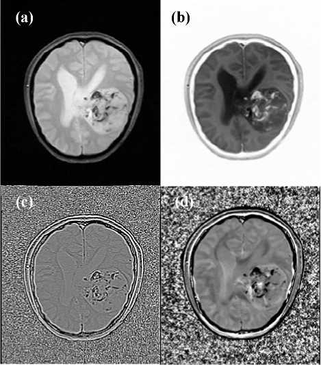
Fig. 6. The Magnetic Resonance Imaging showing the tumor is (a). The image is made of a 416 x 512 pixels matrix with pixel size of 0.49mm x 0.49mm. The Classic-Curvature image and the Intensity-Curvature Functional image are presented in (b) and in (c), (d) respectively. The images in (b) and in (c) were obtained setting the parameter in (1) to the value of -0.54, while in (d) the value of the parameter was set to 2.54. In reference to (d) the tumor is demarcated in its contour and the blood components inside the tumor are highlighted. In (c) the low contrast does not allow to make the same sharp observations although the blood components are visible.

Fig. 6 shows results obtained when fitting the bivariate and the trivariate cubic Lagrange polynomial to the brain image data seen in (a). In (b) is visible the ClassicCurvature image and in (c) and in (d) are visible the Intensity-Curvature Functional images obtained when fitting the bivariate (see (c)) and the trivariate (see (d)) cubic Lagrange polynomials.

The Classic-Curvature image (see Fig. 6b) demonstrates faithful reproduction of the original MRI therefore showing all of the human brain features including the dark spots (fluids) of the tumor which are seen in white color. The Intensity-Curvature Functional image (see Fig. 6c) places the emphasis on what is seen as white spots (fluids) in the Classic-Curvature image (see Fig. 6b) and reproduces them with well-defined level of details. The brain ventricles in Fig. 6b show well demarcated anatomy. As far as the figures in (c) and in (d) are concerned, the Intensity-Curvature Functional acts as a feature extractor of the image seen in (b), therefore showing details (see dark spots) that are seen in both (a) and (b), with a different and complementary perspective. Similar behavior of the Intensity-Curvature Functional images in relationship to the Classic-Curvature images was already observed in both of Fig. 3 and Fig. 4.

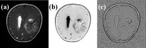
Fig. 7. The Magnetic Resonance Imaging showing the tumor is (a), the image is made of a 484 x 484 pixels matrix with pixel size of 0.41mm x 0.41mm; (b) the Classic-Curvature and (c) the Intensity-Curvature Functional. The images in (b) and in (c) were obtained setting the parameter in (1) to the value of -0.54.

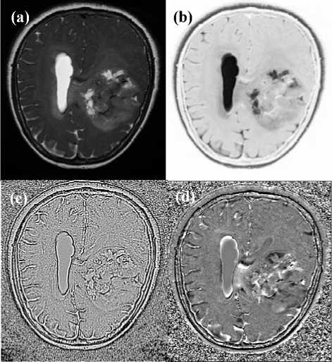
Fig. 8. The Magnetic Resonance Imaging showing the tumor is (a). The image is made of a 512 x 512 pixels matrix with pixel size of 0.39mm x 0.39mm; (b) the Classic-Curvature, (c) and (d) show the IntensityCurvature Functional images. The images in (b) and in (c) were obtained setting the parameter in (1) to the value of -0.54, while in (d) the value of the parameter was set to 2.54. In (d) is visible the mass effect of the tumor pushing the ventricles. Also well visible in (d) are the white components which could be water and/or blood, fluid more in general.

Fig. 7 and Fig. 8 show the original MRI with the tumor in (a), the Classic-Curvature image in (b) and the Intensity-Curvature Functional image in (c). The imaging behavior of the two mathematical engineering tools is similar in both of Fig. 7 and Fig. 8. While the ClassicCurvature shows remarkable reproduction of the original

MRI image features overall all of the anatomical structures, the Intensity-Curvature Functional seen in Fig. 7c and Fig. 8c performs feature extraction from both of the white and dark nuances of the tumor which are visible in Fig. 7a and Fig. 8a.

The area of the tumor is well visible in Fig. 7b and Fig. 8b, whereas the contours of the white and the dark nuances of the tumor are demarcated in the IntensityCurvature Functional of Fig. 7c and Fig. 8c. Fig. 8d shows the Intensity-Curvature Functional obtained when fitting the data with the trivariate cubic Lagrange polynomial. Similarly to what was seen in Fig. 5c, Fig. 8d place the emphasis on the depths of the anatomical structures of the brain and of the tumor.

Generally speaking, the Classic-Curvature images shown in this paper manifest high similarity when compared to the original MRI and therefore behave as information provider to the diagnostic value of the original MRI. The Classic-Curvature images can also appear inverted as far as regards their comparison with the original MRI and such behavior is observable because of the use of a negative value of the constant 'a' in (1). Examples of the aforementioned behavior can be seen in Fig. 6b, Fig. 7b and Fig. 8b. Distinction between gray and white matter of the human brain and highlights on well demarcated brain structures are all possible to achieve with the Classic-Curvature images.

On the other hand, the Intensity-Curvature Functional images tend to highlight the contours, the inner structures of the tumor, such as the white and dark spots, and also are able to provide depth information of the brain structures such as the sulci (see Fig. 8d).

• IV.    DISCUSSION

• A.    The Computational Intelligence

This section discusses how to obtain the ClassicCurvature and the Intensity-Curvature Functional from two-dimensional MRIs. The first step to undertake is that one of fitting a polynomial function to the signal-image data. The polynomial function needs to benefit of the property of second-order differentiability, which is that one that admits the model polynomial function to have non null and continuous second-order derivatives in its interval of definition. The effect of fitting the model polynomial function, to the discrete sequel of digital samples the MRI which is made of, is that of creating the continuum from the digital (discontinuous) nature of an MRI two-dimensional image.

The second step is the calculation of all of the second-order derivatives of Hessian of the polynomial function. This step implies that also the second-order derivatives with respect to the covariates are calculated (for instance x and y) and is the step which provides both of third and fourth steps of the mathematical procedure with the computational intelligence.

The third step is the calculation of the ClassicCurvature, which is possible through the summation of all of the second-order derivatives of the Hessian of the model polynomial function fitted to the signal-image. The calculation of the Classic-Curvature brings the benefit of including into the resulting second-order derivative of the signal-image both of the derivatives in the same variable and the derivatives in the covariates.

Thus, the aforementioned approach advances the state of the art versus approaches which use compact finite differences [9], multidimensional derivative filters [10] to calculate both of first and second order derivatives, and/or gradients [11], and/or the Sobel operator to calculate the first order derivatives of the signal-image [12].

The fourth step is that one of the calculation of the Intensity-Curvature Functional through the ratio between two terms each of which is a composition between pixel intensity and Classic-Curvature of the model polynomial function. The two terms are: (i) the numerator, which is made of the integral of the product between the pixel intensity at the grid node (the value f(0, 0) in 2D, or f(0, 0, 0) in 3D) of the intensity extracted from the discrete sequel of digital samples) and the Classic-Curvature calculated at the grid node ((x, y) ≡ (0, 0) in 2D, or (x, y, z) ≡ (0, 0, 0) in 3D); and (ii) the denominator, which is made of the integral of the product between the pixel intensity at the intra-pixel re-sampling location (x, y), which is (x, y, z) in the three-dimensional case, and the Classic-Curvature calculated at (x, y), which is (x, y, z) in the three-dimensional case. It is therefore important to stress that in the calculation of both Classic-Curvature and Intensity-Curvature Functional the intra-pixel resampling coordinate is another piece of computational intelligence and is also one main determinant of the appearance of the images of the two aforementioned mathematical engineering tools. Another main determinant is the polynomial form of the model function fitted to the signal-image data. A consequence of the intra-pixel re-sampling is that for a given MRI there are an immense number of possible Classic-Curvature and Intensity-Curvature Functional images, each of which is corresponding to the coordinate (x, y) or (x, y, z). This characteristic gives plenty of freedom regarding the calculation and the choice of the Classic-Curvature and the Intensity-Curvature Functional images which allow achieving best diagnostic results.

• B.    The Value Added to the Original MRI

As seen in the results section the characteristics of the Classic-Curvature and the Intensity-Curvature Functional images are those of adding imaging information to the one already available through the observation of the original MRI. It is visible from the figures presented in the results section that the two mathematical engineering tools can highlight various anatomical structures of the human brain. The cortex (see Fig. 3), the sulci and their depths (see Fig. 7c and Fig. 8c, Fig. 8d), the distinction between gray matter and white matter (see Fig. 6b), the ventricles and the Cerebrospinal Fluid (CSF) (see Fig. 3a, Fig. 4b, Fig. 6b, Fig 7b, Fig. 8b), the cerebellum (see Fig. 5b and Fig. 5c) and also sub-cortical structures (see Fig. 3a and Fig. 3b), are all anatomical structures that both the

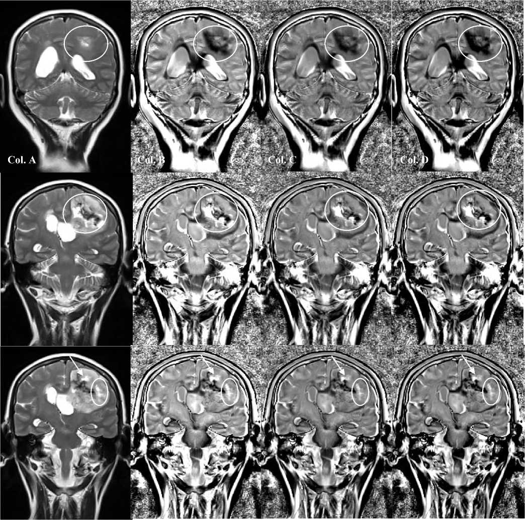
Fig. 9. The original MRI is placed in the left column (Col. A). Three different calculations of the Intensity-Curvature Functional with the trivariate cubic Lagrange formula when re-sampling at: (x, y, z) ≡ (0.1mm, 0.1mm, 0.1mm), see images in the second column from right (Col. B); (x, y, z) ≡ (0.5mm, 0.5mm, 0.5mm), see images in the third column from right (Col. C); and (x, y, z) ≡ (0.9mm, 0.9mm, 0.9mm), see images in the left column (Col. D). All of the images are brightness-contrast enhanced.

Classic-Curvature and the Intensity-Curvature Functional images can reproduce. It is also possible to have confirmation of an anomaly such as the tumor as studied in this paper. Most importantly, though, the ClassicCurvature and the Intensity-Curvature Functional images can perform feature extraction from the original MRI. Specifically, what was already seen in Fig. 3b, Fig. 4b, Fig. 5c, Fig. 6d, Fig. 7c and Fig. 8d, remark that the Intensity-Curvature Functional extracts features which are seen under a different perspective when compared to the information provided with the original MRI.

Additionally, Fig. 7c, Fig. 8c and Fig. 8d serve as example of the behavior, shown by the IntensityCurvature Functional images, which emphasizes on the depth and the length of the brain sulci in a manner which is different from the depth perceived when visually inspecting the original MRI.

In the present research, the emphasis is on the collection from the tumor of information which is not readily observable through the original MRI. Thus, through the use of the Classic-Curvature and the Intensity-Curvature Functional, it is possible to extract features from the original MRI. The process of feature extraction is enhanced because the Classic-Curvature and the Intensity-Curvature Functional can be calculated at an enormous number of intra-pixel coordinates of the MRI images. Each time the two mathematical engineering tools are calculated, the signal-image is re-sampled through the model function fitted to the signal-image. Therefore, the computational intelligence provided with re-sampling (which is inherent to the calculation of the two mathematical engineering tools) makes it possible the tuning of the property of feature extraction from MRI images. Thus it is possible the collection of information from the tumor, which is complementary to the information provided with the original MRI.

In order to investigate the effect of the change of the intra-pixel coordinates where the signal is re-sampled, the experiment shown in Fig. 9 was performed using the trivariate cubic Lagrange formula. The MRI volume was re-sampled at the intra-voxel coordinates: (x, y, z) ≡ (0.1mm, 0.1mm, 0.1mm), (x, y, z) ≡ (0.5mm, 0.5mm, 0.5mm) and (x, y, z) ≡ (0.7mm, 0.7mm, 0.7mm). The images in the top row of Fig. 9 generally show that the Intensity-Curvature Functional reconstructs the tumor structure quite faithfully regardless of the intra-voxel coordinates used for re-sampling (see inside the white ellipses), although the image re-sampled with (x, y, z) ≡ (0.1mm, 0.1mm, 0.1mm) (see the second image from left in top row) is slightly more accurate than the other two. The Intensity-Curvature Functional seen in the second row from the top shows to be very much alike in the reconstruction of the MRI (except for the brightnesscontrast enhancement) for all of the three intra-voxels coordinates (see the tumor region enclosed in the white circle). The images in the bottom row in Fig. 9 show that none of the three intra-voxel coordinates, used for resampling and for the calculation of the IntensityCurvature Functional, make the reconstruction of the tumor structure accurate (see the white arrow). Whereas the tumor structure inside the white ellipse in the bottom row is satisfactorily reconstructed when using all of the re-sampling intra-voxel coordinates.

To place the research herein presented within the context of the literature, it is due to acknowledge the interdisciplinary nature of the research. Our research intersects with biomedical informatics [13] as well as with biomedical image processing [14], and biomedical feature extraction from the pathological human brain [15].

• C.    Benefits and Limitations

The behavior of MRI feature extraction is certainly a benefit which originally descends from the process of fitting the polynomial function to the digital sequel of MRI samples. The mathematical process to obtain the Classic-Curvature and the Intensity-Curvature Functional is somehow lengthy and needs extra attention because of the non-trivial application of calculus and algebra. This process can be considered a limitation because it makes complex the calculation of the mathematical engineering tools. The coding of the math of both Classic-Curvature and Intensity-Curvature Functional is also a limitation because of the complexity of the math formulae.

Nevertheless, the most precious advantage of this piece of research, which is related to a larger research project published recently in [6], is that the feature extraction behavior of the Classic-Curvature and the IntensityCurvature Functional can contribute to diagnostic radiology. The contribution is within the context of the analysis of medical images in Magnetic Resonance Imaging and it is determined through the herein presented computational intelligence approach.

• V.    CONCLUSION

In the study presented in this paper, the characteristics of the MRI of the human brain which are given as complementary information to the MRI are: (i) the contour line of the tumor (see for instance the IntensityCurvature Functional image in Fig. 3b), (ii) the pressure on the ventricles exercised by the tumor (see for instance the Intensity-Curvature Functional image in Fig. 4b), (iii) presumed brain vessels shown in the original MRI (see Fig. 5b, which is a Classic-Curvature image and Fig. 5c, which is an Intensity-Curvature Functional image), (iv) liquids of the tumor (see Fig. 6b and Fig. 8b, which are Classic-Curvature images, and Fig. 6d and Fig. 8d, which are Intensity-Curvature Functional images), and (v) the overall structure of the tumor with a shaded region enclosing the pathology (see Fig. 7b, which is a ClassicCurvature image).

Acknowledgment

The software is available from the corresponding author at no charge whatsoever. This work presents a case study on a patient suffering from brain tumor. The MRI scans were collected after proper administration of the informed consent to the patient and in agreement with ethical committees of the Skopje City General Hospital. The authors are grateful to Ms. Monica Chiang because of the coordination of the paper submission, to the anonymous reviewers because of their useful suggestions aimed to improve the paper, and to the MECS Publisher editorial team because of the excellent typesetting of the paper.