Computing the Bodies Motions in the Space and Long-term Changes in the Earth's Climate

Published Online December 2019 in MECS DOI: 10.5815/ijmecs.2019.12.04

• I.    Introduction

  In 2018, two monographs [1] and [2] were published, based on the results of solving problems of interaction between bodies and the evolution of their movements. The problems were being solved within several decades. The movement of the bodies of the Solar system,

including Earth, Mars, Mercury, asteroids and other bodies, was investigated. Also the movement of the bodies that make up the constellations was investigated. Tasks were considered, both translational and rotational. As a result, a new understanding of the processes occurring on the Earth and in the Solar System has been obtained. This paper has reviewed the results of these two books. The main result is long-term climate change on Earth. It is due to the interactions of the bodies of the Solar system.

All results presented in the paper were obtained by the author. The paper is intended for a wide circle of readers to familiarize them with the latest scientific results. It is especially useful for students and young researchers who know computer methods. The paper has many examples, following which they can perform their term papers and dissertations.

• II.    The book “FUTURE Space Problems and Their Solutions”

  • 2.1.    The book cover

• 2.2.    The Researcher’s Comments

  • 2.2.1.    Academician Vasily M. Fomin, one of the leaders of the Siberian Branch of the Russian Academy of Sciences

• 2.2.2.    Prof. Vladislav V. Cheshev, the great philosopher from Tomsk, Tomsk State University, Russia

The front cover in book [1]shows 50 such planets like the Earth, which are located on a sphere around the Sun. They make a revolution in 1 year and receive as much solar heat as the Earth is now. This is the result of an exact solution to the problem of the interaction of bodies uniformly located on a sphere. It provides unlimited opportunities for the development of Mankind [3].

The author is presented on the back cover [1] during a presentation at the Madrid exhibition on May 14, 2011, about the Galactica system, which is intended for solving problems of gravitational interaction of bodies.

Before the Content of the book are comments of scientists about it.

The manuscript of J.J. Smulsky's book "Future space problems and their solutions" appeared in my hands. Everyone, sitting at a fire, admired the nature surrounding us on the Earth and the starry sky of our Universe, its abundance of stars, planets, asteroids and comets. And always the question arose, how they move, what interactions between them occur. That is way this book is devoted to the calculation of bodies’ movements in various cases of interaction, based on gravitational forces. The developed system "Galactica" [1, 4 - 6] has free access and is designed for numerically solving the problems of gravitational interaction of N-bodies. As a result of working with this system, one can study the optimal movements of spacecrafts, the evolution of the Solar system for 100 million years, the influence of the Sun on the Mercury’s perihelion, the evolution of the Earth's rotation axis and much more, which allows us to gain new knowledge about our world.

The system "Galactica" is well described and allows the user with higher education to work with it. All calculation results are displayed for convenience on the display screen. Using this system, the trajectories of asteroids "Apophis" and "1950 DA", their possible approaches to the Earth are studied and various ways of transforming these trajectories are indicated.

Thus, the reader will find a lot of interesting and will be able to explain some of the phenomena that occur in the long-term climate change on Earth, the formation of the future habitat of mankind. Maybe some insights will not coincide with existing conceptions at this time; however, they will serve as a basis for further research in this interesting field of knowledge.

Today it is customary to speak of the Universe as a product of the Big Bang, which gave rise to the mystery of dark matter, expanding Universe and other tempting but badly comprehend realities. Joseph J. Smulsky gives the chance to feel the harmony of the world, to see it in the image of reasonable classical simplicity peculiar to Isaak Newton's mechanics. The elegance of simplicity and the complexity of the system appear in their mathematically comprehended unity.

• 2.2.3.    Doctor of Technical Sciences Boris F. Boyarshinov,Insitute of Thermophysics, SB RAS, Novosibirsk, Russia

• 2.2.4.    Dr. Sc. in Physics and Mathematics Michael P. Anisimov,Head of the Nanoaerosol Laboratory, SB RAS, Novosibirsk, Russia; Research Professor, Clarkson University, NY, USA

• 2.2.5.    Doctor of Technical Sciences Nikolay E. Shishkin, Insitute of Thermophysics, SB RAS, Novosibirsk, Russia

• 2.3.    Foreword

  Over a period of fifty years, Professor Joseph J. Smulsky has been successively developing and bringing into fruition a novel method for reality cognition. He called his method a hypothesis-free method. The method was described in a book titled “The Theory of Interaction”, issued in 1999 [4]. According to J.J. Smulsky, the action of one on another body consists in that the second body starts moving with acceleration. Mankind has developed mechanics, a science in which the interactions are measured as forces and the acceleration of a body is expressed in terms of the force and the relation between this body and some standard body called mass. By dividing the force by mass, we obtain the body’s acceleration. All forces and masses can be measured, and both the interactions among the bodies and the bodies’ motions can, therefore, be calculated.

The problems of gravitational interaction of bodies are extremely diverse. The author considers the situations most significant for the space exploration and to the preservation of life conditions on the Earth-planet. The developed program Galactica can be of interest for professionals and students of the relevant specialties, as for as it allows to apply the received data for the analysis of various problems of celestial mechanics.

The book is very impressive. Prof Joseph J. Smulsky considers grandiose projects: the optimal approach of the spacecraft to the Sun, the transformation of asteroids into satellites of the Earth, the creation of new planets like the Earth etc. Without doubt that the space agencies will use the solutions and soft, which are discussed and presented in the book. That will raise the computation culture in the area under consideraion.

Environment and human well-being are due to many factors, including the influence of movements of cosmic bodies both in the Solar system and beyond. The proposed monograph provides an excellent opportunity to predict the motion and rotation of planets, to optimize the flights of spaceships by means of a sufficiently simple to assimilate the program Galactica. A lot of worries are caused by possible collisions of comets and asteroids with the Earth. The examples of the most dangerous two asteroids show the capabilities of the Galactica program to calculate their evolution. These opportunities are wider than they are presented in the book. But even what is given impresses with its multifaceted tasks and their scale.

After the Contents, there is a preface to the book, in form of the Foreword, written by Vitaly F. Novikov, a professor at Tyumen Industrial University. He is familiar with the author’s works because for several decades Novikov V.F. repeatedly was a reviewer of Smulsky’s monographs.

In this approach, no presumptions or hypotheses about the nature of the interactions are necessary: it does not matter why the interactions exist, how they are transferred, and so on. That is why many theories such as the gravitational theory, the space-time theory, and the theory of relativity turn out to be unnecessary structures.

In the present book, the hypothesis-free method was employed to study the motion of space bodies. For calculating the interactions, J.J. Smulsky has developed software Galactica [1, 4 - 6], which allows one to solve, with high accuracy, problems that could not be solved previously. One of such problems, for instance, is the evolution of the Solar system for 100 million years.

Also, J.J. Smulsky has analytically exactly solved some previously unsolved N-body problems, including the following ones: what motions are exercised by bodies on a ring [7]? Can a system of bodies involving several of rings rotate as an entity [8]? Those and other exact solutions have allowed J.J. Smulsky to solve several previously unsolved problems: about an optimum mission to the Sun [9], about the motion of Mercury’s perihelion [10], about the evolution of the Earth axis [11, 12], and so forth.

The solutions obtained provide new impressions of our world, explaining why the climate on the Earth suffers changes and what achievements are possible for mankind in the future.

In his new book, Smulsky explains the solution to these problems, provides detailed proofs, solution methods, computer programs and initial data. The whole toolkit allows young researchers to retrace the path of the pioneer of the problems presented, as well as to attempt the solution of unsolved other problems.

Vitaly F. Novikov,

• 2.4.    Some book’s findings

Periodic changes are taking place on the Earth: day gives way night, and winter comes after summer. There are also more significant changes when the climate gets colder, and Ice Ages begin, and then followed by warm periods. We know that the change of day and night times on the Earth is caused by the rotation of the Earth around the Sun, and the change of seasons is due to the Earth's orbital motion. Apparently, the longer-term changes are also due to the changes in the motion of Solar-system bodies. After several years of working on that problem, the author has developed the following research plan (Fig. 1). First, it is necessary to study the evolution of the orbits of the Solar system bodies and, then, the evolution of the axis of Earth’s rotation. At the third stage, it is required to investigate the evolution of insolation, and at the fourth, to compare the change in insolation with the change in natural processes. Then, at the fifth stage, we can finally tell how natural processes will develop on the Earth.

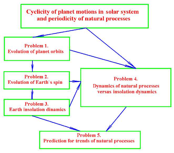
Fig.1. The problems and relationships between them in the study of the evolution of the Earth’s Cryosphere as a result of the interaction of Solar system bodies [13].

The graphs (Fig. 2) show the changes of the four parameters of the Mars orbit: the eccentricity e , the angle of the orbit’s node ϕ Ω , the inclination angle of the orbit plane i , the perihelion angle ϕ p , and the perihelion’s angular velocity ω p over two time intervals, each interval lasting 50 million years. Such parameters are given in Fig. 2: T_e2 is the second period of eccentricity, T_Ω and T_i are the shortest periods ascending node and inclination, respectively, in kyr (thousand years); e_m , i_m and ϕ_Ωm are the average values of appropriate parameters; T p is a rotation perihelion period averaged over 50 Myr.

The parameters of the Mars orbit fluctuate within unchanged limits. The graphs showing the data over the two intervals of 50 million years are almost indistinguishable. Thus, the Mars orbit is regular and stable, and there are no signs for the violation of this stability. The same results were obtained for the other planets [13]. These results, therefore, prove the stability of the entire Solar system.

Before the author’s work, the researchers came to the conclusion about the instability of the Solar system and about its possible destruction in one billion years. The graph (Fig. 3) by Laskar and co-authors shows that the angle of inclination of the Mars orbit may change irregularly and, depending on the initial conditions, those changes may follow any of the four variation patterns.

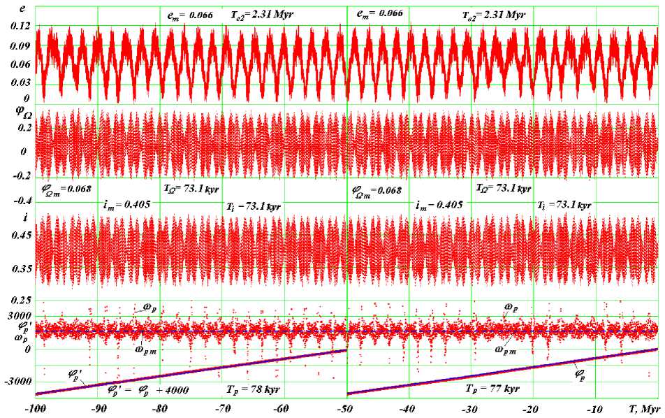
Fig.2. The evolution of the Mars orbit in the span of 100 million years: T is the time in millions of years into the past from the epoch 30.12.1949. w pm = 1687 "/century is the average angular velocity of the perihelion [14].

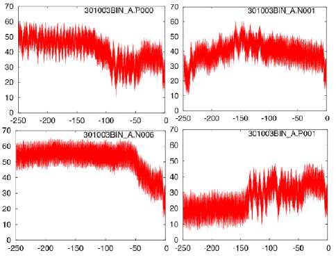
Fig.3. The angle between the planes of the orbits of Mars and its equator at different initial conditions in the solutions by Laskar et al. [15]: the angle ( Y -axis) is in degrees, and the time ( X -axis) is in the past 250 million years.

These graphs (Fig. 4) show the optimal trajectories of the spacecraft’s approach to the Sun. The position of the bodies, the Earth, Venus, Mercury, and the Sun, is shown by the moment of launch. The spacecraft is launched against the Earth’s orbital motion, and then it moves with the propulsor off. At the end of the propulsor’s operation, the coordinates and the velocity of the spacecraft are calculated so that it would have passed at a certain distance from Venus, letting the Venus to reduce its speed.

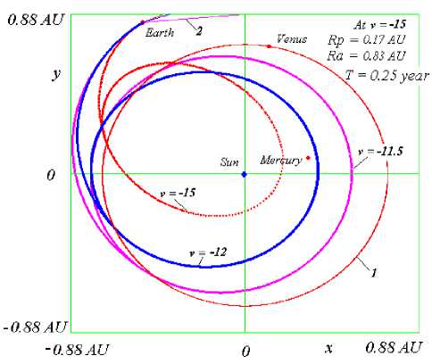
Fig.4. The trajectories and orbits of the spacecraft when launched on January 20, 2001, with different initial velocities v . The flight is passive. After the influence of Venus (when it crosses its orbit), the device goes into an elliptical orbit. 1 is the orbit of Venus [9].

Thus, here (Fig. 4), a closer passage of the spacecraft to the Sun is ensured in comparison with those that can be achieved using other launching schemes. The time required for reaching the closest distance to the Sun is also shortened. For example, with a launch speed of 15 km/s, this time is equal to 0.25 years, whereas, with other launching schemes, this time turns to be equal to several years.

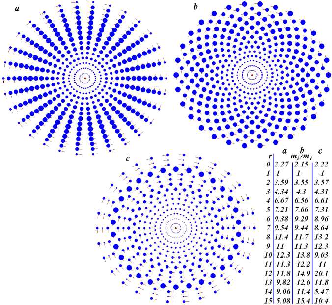
Fig. 5. Images of axisymmetric multilayer rotating structures as displayed on the computer screen. The structures were obtained by integration of differential motion equations performed using the Galactica program: N 2 = 15; N 3 = 30; period P rd =1 year; the mass of the central body is equal to the Sun mass. Given in the table are the relative radii of the rings and the masses of one body in the rings [8].

Here (Fig. 5), results of an exact solution of the problem of N -bodies located in N 2 layers around a central body are shown. Each of the layers contains N 3 bodies, and the whole system rotates as a single entity. In this figure, we see three configurations of such a structure depending on the location of the bodies in adjacent layers. The structures have 15 layers with 30 bodies locating in each layer.

The graphs (Fig. 6) show the distances between the asteroid Apophis and the Mercury, Venus, Moon, Earth and Mars for 100 forthcoming years ( a ), 100 past years ( b ) and 1000 future years ( c ) [16]. In Fig. 6, T in cyr (1 cyr = 100 yr) is the time in Julian centuries from November 30.0, 2008. Calendar dates of approach in points: A – April 13, 2029; B – April 13, 2067; C – September 5, 2037; E – October 10, 2586.

At the moment A , April 13, 2029, Apophis will pass at a distance of six Earth’s radii, and there will be no more such approaches. Therefore, during the execution of this work in 2011, we proposed to transform the trajectory of Apophis into the orbit of an Earth satellite.

The same studies were performed for the asteroid 1950 DA, weighing 30 times more than Apophis. The asteroid 1950 DA will pass after 600 years at a distance from the Earth no closer than 2 million km.

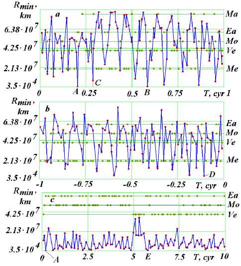
Fig.6. Apophis’s encounters with celestial bodies during the time Δ T to a minimum distance Rmin, km: Mars (Ma), Earth (Ea), Moon (Mo), Venus (Ve) and Mercury (Me); a , b – Δ T = 1 year; c – Δ T = 10 years.

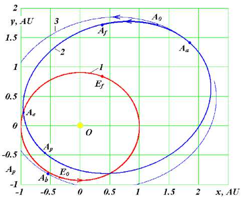
Fig.7. The trajectories of Earth ( 1 ) and 1950 DA ( 2 ) in the barycentric equatorial coordinate system xOy over 2.5 years in the encounter epoch of March 6, 2641 (point A e ): A0 and E 0 are the starting points of the 1950 DA and Earth trajectories; A f and E f are the endpoints of the 1950 DA and Earth trajectories; 3 - 1950 DA trajectory after the correction applied at the point A_a is shown approximately; the coordinates x and y are given in AU.

Fig. 7 shows a diagram of transformation of the trajectory of 1950 DA into the orbit of an Earth satellite. 1 is Earth's orbit; 2 is 1950 DA’s orbit. At the point Aa, the asteroid accelerates slightly, and it bypasses the Earth from the night side, point Ab, at a distance of six Earth’s radii. At the latter point, 1950 DA gets decelerated and becomes a satellite in a geostationary orbit. In this orbit, the asteroid will immovably hang over a certain equatorial point of the Earth.

The graphs (Fig. 8) show the results of calculations of the changes in the parameters of the Mercury orbit due to the interaction of the bodies in the Solar System for two cases: on the left, all bodies are treated as material points, and on the right, the oblate shape of the Sun is taken into account in the form of its 15th model.

Here, points 1 show the calculated parameters for six thousand years, i.e., for spans of ± 3 thousand years from the contemporary epoch; and lines 2 and 3 , the results of approximation of the observational data.

The following parameters were considered: the eccentricity e , the inclination angle of the orbit plane i , the angle of the orbit’s ascending node ϕ Ω , and the perihelion angle ϕ p . All these parameters suffer changes. Since two other parameters, the major semi-axis a and the period P undergo no changes, the oscillations of the deviations of those parameters, Δa and Δp are shown here.

A noticeable difference between the calculated and observational data is only observed for ϕ p0 . As seen from the right graph, taking into account the oblate shape of the Sun leads to the coincidence between the calculated and observational data.

Thus, the Newton law of gravitation allows one to rather accurately predict the motion of all bodies in the Solar system.

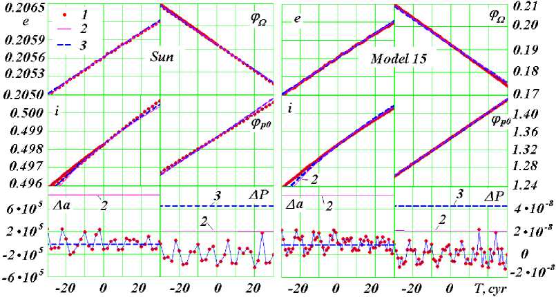
Fig.8. A comparison of the results of integrating differential equations of the Solar System bodies interaction in a span of 6,000 years with the form of point Sun (left) and with a compound model No. 15 (right) for the secular changes of the Mercury’s orbital elements. The interval between the points in centuries is two for left graphs and one for the right graphs; e is the eccentricity; i is the angle of inclination of the orbit plane to the equator plane of 1950.0; ϕ Ω is the angle of the ascending node of the orbit; ϕ p0 is the angle of the perihelion; Δa in m is the semimajor axis deviation from the average of 6,000 years, the values in meters; ΔP in centuries is the orbital period deviation from an average of 6,000 years. The angles are in radians, and the time T is in centuries in the past and the future from the epoch December 30.1949. 1 shows the results of the numerical solution of the

Galactica program; 2 shows the secular changes according to S. Newcomb, 1895 [17]; and 3 shows the secular changes according to J.L. Simon et al., 1994 [18].

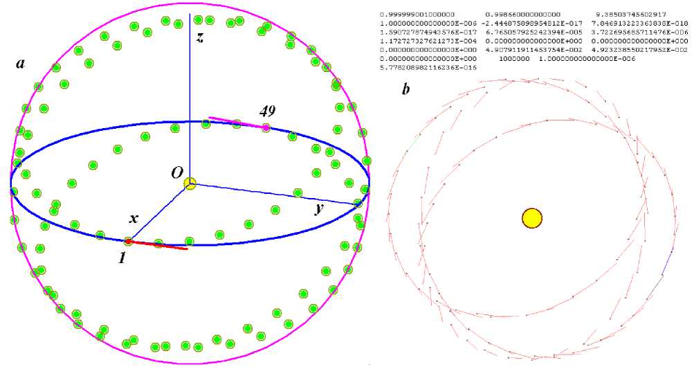
Fig.9. A regular spatial structure with N = 100, radius of the sphere R = 1 AU (astronomical unit is equal to 1.496 million km), and period P rd = 1 year and with the central-body mass equal to the Sun mass: a – in 3D coordinate system, the lines at bodies 1 and 49 indicate the velocity vectors; b – image of the structure as displayed on the computer screen after 100 revolutions of a peripheral body around central body in the integration of the differential motion equations (1.3) with the Galactica system; a – projection onto the frontal plane, b – projection onto the horizontal plane.

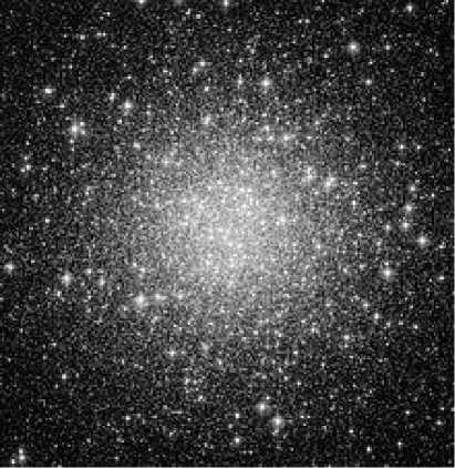
Fig.10. The M 53 (or NGC 5024) globular star cluster in the Coma Berenices constellation

The Fig. 9 shows a structure formed by 99 bodies uniformly distributed on a sphere around the Sun. This structure was obtained as a result of the exact solution of the interaction problem of these bodies. The bodies are evenly distributed along the three-turn curve. On the right, these bodies are shown in motion. Each body moves in a circular orbit, and it receives as much heat from the Sun as the Earth presently does. As it is already noted, the results obtained while solving this problem offer unlimited possibilities for the development of mankind.

Fig. 10 shows a globular star cluster in the Coma Berenices constellation. The globular star clusters are the oldest formations in the universe. Thousands of stars move in their orbits and never collide. How does this happen?

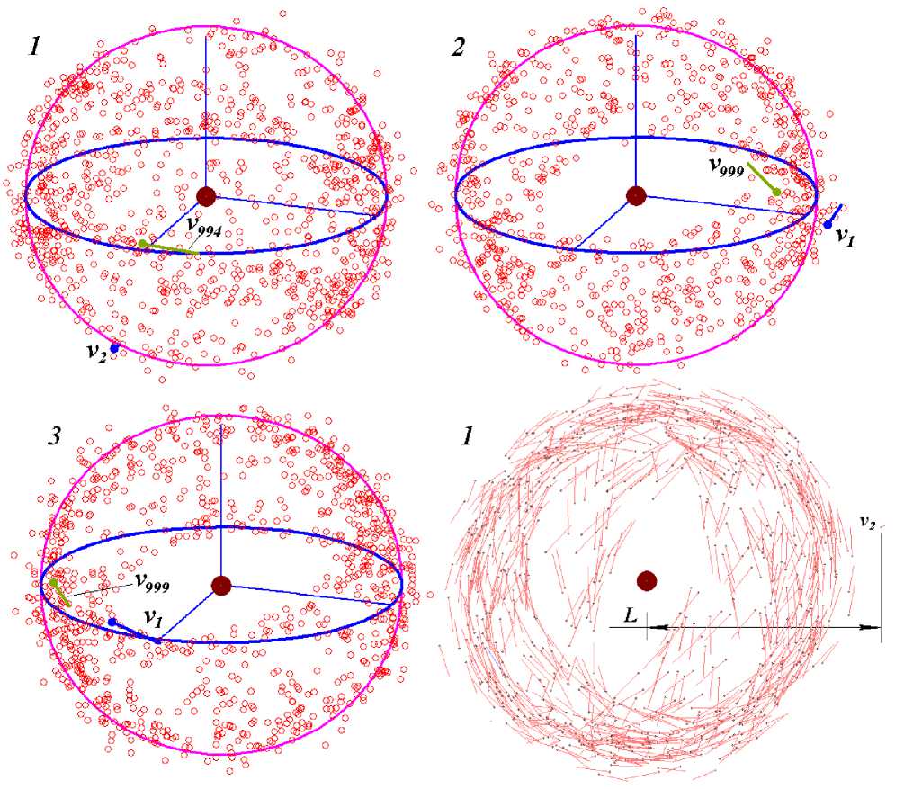
Fig.11. Spherically distributed structures with N ≈ 1000 after 100 revolutions of the peripheral bodies: 1 , 2 , and 3 — versions of the initial structures. Bottom right shows structure 1 in motion. The line bars at bodies 1 and 999 and so on indicate their velocity vectors v 1 and v 999 . The distance L to the second body is been diminished in 2 times.

Fig. 11 shows three models of globular star clusters, which were derived from the spherically distributed solutions. This images are the models appearance after 100 revolutions of each body. After 50 revolutions, the configuration does not change. The models differ in the formation scenarios of the spherical structure. Structure 1 is shown in dynamics in the right bottom. The body 2 has an elongated orbit. In the dynamics, it becomes evident that the bodies move at differently directed velocities. At the beginning of the formation process, some of the bodies suffer collisions, and some of them merge into one body. The bodies become larger; as time passes, the collisions grow rare, and there comes a time when no further collisions occur. Each body acquires its own orbit close to an ellipse. The plane of this orbit intersects the planes of the orbits of other bodies, but the bodies pass the common points of their orbital planes at different places or at different times.

In contrast to the globular clusters shown in Fig. 10, in these models (Fig. 11) the bodies are concentrated at the periphery. Such globular clusters are also found.

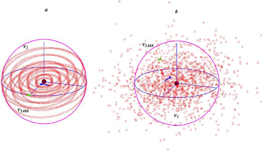
Fig.12. Multilayer spheroidal model of a globular star cluster: shown are five layers involving 1488 peripheral bodies; a — at the time the structure was formed; b — after the 196th revolution of the first-layer body; the line bars at bodies 1 and 1488 indicate their velocity vectors, v 1 and v 1488 .

The model of a spherical star cluster is developed based on a multilayer structure (Fig. 12). The figure on the right shows this structure after 196 revolutions of the bodies in the inner layer. The structure was formed after the 20th revolution, and during further 180 revolutions it remained almost unchanged.

• III.    The book “NEW Astronomical Theory of the Ice Ages”

  • 3.1.    The book cover

• 3.2.    Annotation

3.3. Some book’s findings

The front side of the cover [2] shows how the Earth's illumination by the Sun is related to the orbital and rotational motion of the Earth (Fig. 13). The Earth rotates around its axis, and therefore there is a change of day and night times on it. Rotation proceeds in a counterclockwise direction. The Earth moves around the Sun in its orbit also counterclockwise. The Sun is located not at the center of the orbit, but in one of the foci of the ellipse. Therefore, in perihelion (in winter, the Northern Hemisphere), it approaches the Sun to the smallest distance R p , and in aphelion (in summer) it moves away from the Sun to the greatest distance R a . The axis of the orbit S is perpendicular to its plane. The axis of Earth’s rotation N is inclined to the Earth axis at an angle of 23.4°. Therefore, on December 21, the Southern Hemisphere is better illuminated by the Sun, and the polar night stands behind the Arctic Circle. This is the winter solstice. On June 21, the Northern Hemisphere is better illuminated, and the polar day is above the Arctic Circle. At the position of March 20 and September 22, both hemispheres are equally illuminated. This is the day of the spring and autumn equinoxes, respectively. This is how the seasons change.

The parameters of the orbital and rotational motions of the Earth at the contemporary epoch create the climate on Earth that we know. However, these parameters undergo changes. The axis of the orbit S rotates, or precesses, around the vector MM clockwise, while the Earth’s axis N precesses also clockwise around another vector MM . Also, the both axes oscillate. Additionally, the orbit, shaped like an ellipse, rotates in its plane counterclockwise, and its shape changes: the ellipse either becomes more elongated or its turns into a circle. All this leads to climate change on the Earth, and it becomes the one we do not know yet. The back cover of the book contains the book’s annotation.

The commentary of the scientist about "New Astronomical Theory of the Ice Ages" can be viewed in its review by Prof. Vladimir E. Zharov [19].

This book examines the factual aspects of the following problem: how our world works, why the observable phenomena occur, and why they evolve. The problems of the evolution of the orbital and rotational motions of the Earth, which underlie the new Astronomical theory of the ice ages, are among the most difficult problems in contemporary science. These problems were solved, and the book presents the obtained results, which can be comprehended by a wide circle of the readers. The comprehensibility of the book has been achieved due to 63 drawings and graphs, which also make the book compact and informative. The material contained in the illustrations far exceeds the text of the book, and it will serve as the basis for further research in various fields of science. For those who wish to understand the origins of the results obtained, to check and verify their validity, and maybe even obtain them themselves, the book is supplemented with the material given in Appendices.

Consider the periods during which the parameters of the orbital and rotational motions chang (Fig. 13). The oscillation periods of the orbit’s axis S are: 97.35, 1164, and 2320 thousand years [20].

Eccentricity is

e =

R a

—

R p

/R a + R p '

Oscillations periods of e are: 94.5, 413, 2310 thousand years.

The average period of perihelion’s rotation is 147 thousand years.

The orbit’s axis S (Fig. 13) precesses around the vector MM clockwise with a period of 68.7 thousand years, and the Earth’s axis N also precesses clockwise around the vector M₂ with a period of 25.74 thousand years.

The periods of oscillation of the Earth’s axis N are: 1 day, half a month, half a year, 18.6 years, and tens of thousands of years.

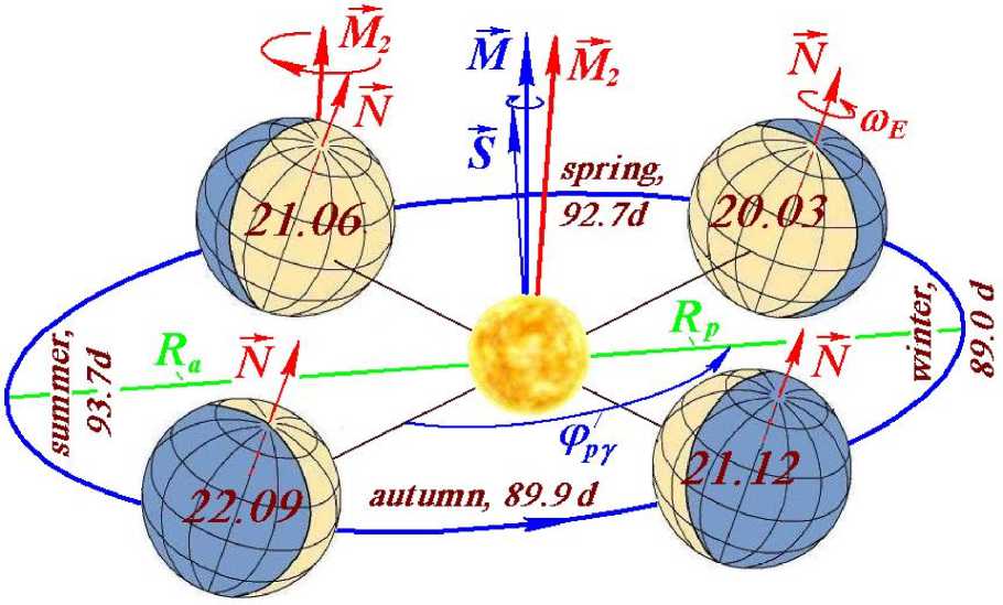
Fig.13. The Earth's position in its orbit in 2025 at the days of the spring equinox (March 20), of the summer solstice (June 21), of the autumn equinox (September 22) and of the winter solstice (December 21), and the time of its movement in days in spring (92.7 d), in summer (93.7 d ), in autumn

*                                                                                             *                                                                                                   *

(89.9 d) and in winter (89.0 d): N is the Earth’s axis of its rotation, and M is the vector, relative to which the axis N precesses with a period of

25.74 thousand years; S is the axis of the Earth's orbit, and M is the vector relative to which the axis S precesses with a period of 68.7 thousand years [2].

The amount of heat coming from the Sun to the Earth, i.e. insolation of the Earth, depends on the parameters of its orbit relative to the moving equatorial plane, and is determined by the following parameters: eccentricity of

the orbit e , obliquity ε , which is the angle between the axes S and N (Fig. 13), and the perihelion angle φ pγ .

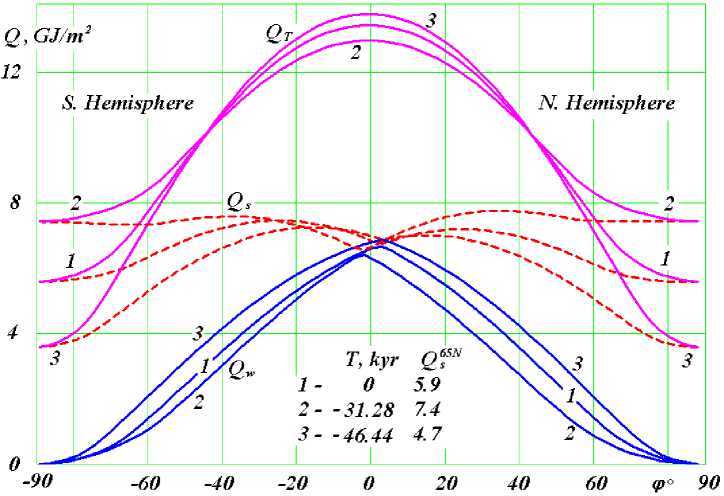
Fig.14. φ -latitude distribution of summer Q s , winter Q w and total, i.e. annual Q T insolations for three epochs: 1 is contemporary one; 2 is the warmest; 3 is the coldest epoch for 200 thousand years ago; Q s⁶⁵N is insolation in GJ/m ² for the summer caloric half-year at the northern latitude of 65 ° ; T , kyr is time in thousand years from d ecember 30, 1949. [2].

The graphs (Fig. 14) show the change in the amount of heat along the Earth's latitude φ from the South Pole (φ = -90°) to the North Pole (φ = 90°) in three epochs over the past 200 thousand years: 1 – contemporary epoch, 2 – the warmest epoch, occurred 31.28 thousand years ago, and 3 – the coldest epoch, which occurred 46.44 thousand years.

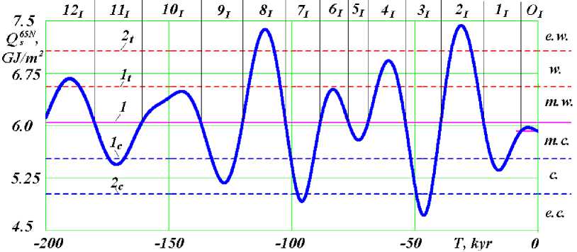
Fig.15. Insolation periods O I , 1 I , 2 I ,…, 12 I over the last 200 kyr and their bounds: 1 is mean insolation Q sm ; 1t and 2t are first and second boundaries of warm levels; 1c and 2c are first and second boundaries of cold levels; m.w., w. and e.w. are moderately warm, warm and extremely warm levels; m.c., c., and e.c. are moderately cold, cold and extremely cold levels [21].

The dashed red lines (Fig. 14) show that from cold epoch 3 to warm epoch 2 , the amount of heat per summer half-year ( Q s ) at the poles had changed two-fold. The range of the variation as we move toward to the equator decreases, and at the equator, the change in heat over the summer half-year is insignificant.

The blue lines show that, during cold epoch 3 , the Earth receives a greater amount of heat in winter halfyear ( Q w ) in comparison with warm epoch 2 . Warmer winters in cold epochs occur over all terrestrial globe.

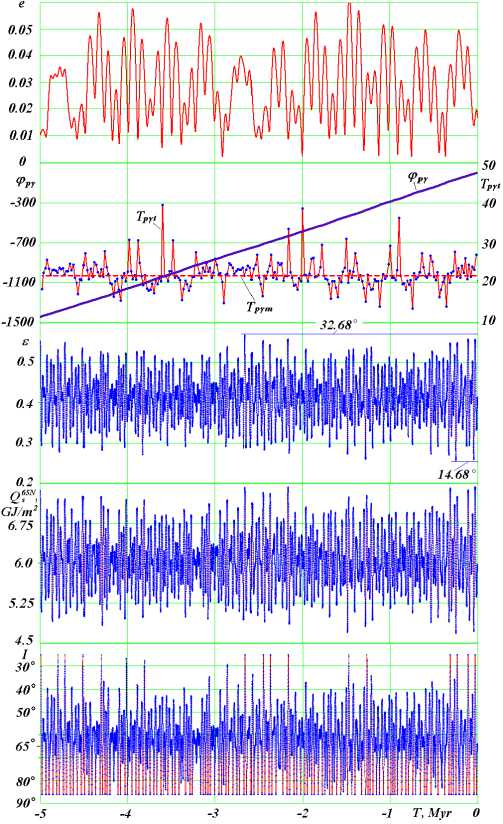
Fig.17. The evolution of the orbit eccentricity e , the perihelion position angle φ pγ , the obliquity ε , as well as the summer insolations Q s ^{65 N} and I for 5 Ma (million years ago); T pγt , thousands years, is a moving average perihelion rotation period for 20 thousand years; T pγm = 21.7 thousand years is the average period of the perihelion rotation.

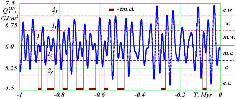
Fig.16. Climate change levels for 1 Myr: 1 - average insolation Q sm ; 1t and 2t - the first and second boundaries of warm levels; 1c and 2c are the first and second boundaries of the cold levels; m.w. , w. , and e.w. are warm levels; m.c. , c. , and e.c. are cold levels; tm.cl. is periods of temperate climate.

The orange lines (Fig. 14) show that from cold epoch 3 to warm epoch 2, the amount of heat per year (QT) at the poles, as well as in the summer half-year, changes twofold. However, the range of change rapidly decreases as we move to low latitudes, and at the latitude of 45 , the annual amount of heat does not change. In the equatorial latitudes, the annual heat changes in the opposite way: in cold epoch 3 at the equator it is warmer than in the warm epochs.

So, first, the warming periods and the cooling periods such as the ice ages occur on the Earth at high latitudes. At low latitudes, in the glacial periods, becomes warmer.

Second, the winters during the glacial periods are warmer than those during the warm periods. These are the climates that exist on the Earth, and which we do not know.

The graph (Fig. 15) shows the changes in heat over the summer half-year at the latitude of 65 degrees in the Northern Hemisphere ( Q s ^{65 N} ) for 200 thousand years ago. The parameter Q s ^{65 N} is an indicator of climate change at high latitudes. All the extremes of Q s ^{65 N} are numbered, the insolation periods 0 I , 1 I ,…12 I of climate change are introduced, and their boundaries are identified. Those periods correspond to: 0 I – Holocene optimum, 1 I – Sartan ice age in Western Siberia, 2 I – Karginsky warming, 3 I – Ermakovsky ice age. The Ermakovsky ice age is one of the strongest glaciations in the past 200 thousand years.

These periods also occur in Europe and North America. However, in those parts of the world, they are called differently [21] – [22].

Also, three levels of warm climate are introduced (Fig. 15): a moderately warm climate, a warm climate, and an extremely warm climate. Similarly, three levels of cold climate are introduced; these are a moderately cold, a cold, and an extremely cold climate.

From the graph (Fig. 16) it is seen that, over the past million years, there have been four extremely warm periods and six extremely cold periods. Those periods occur unevenly. During the first 300 thousand years, all strong cooling and warming periods had occurred. And then there were no such strong changes over the next 700 thousand years.

The graphs (Fig. 17) show the changes in the parameters of the orbital and rotational motion of the Earth and insolation during the past 5 million years; those parameters are the eccentricity e , the perihelion angle ϕ p γ reckoned from the moment of equinox (Fig. 13), the angle e between the axes 5 and N , the summer insolation Q s ^{65 N} and insolation I in equivalent latitudes.

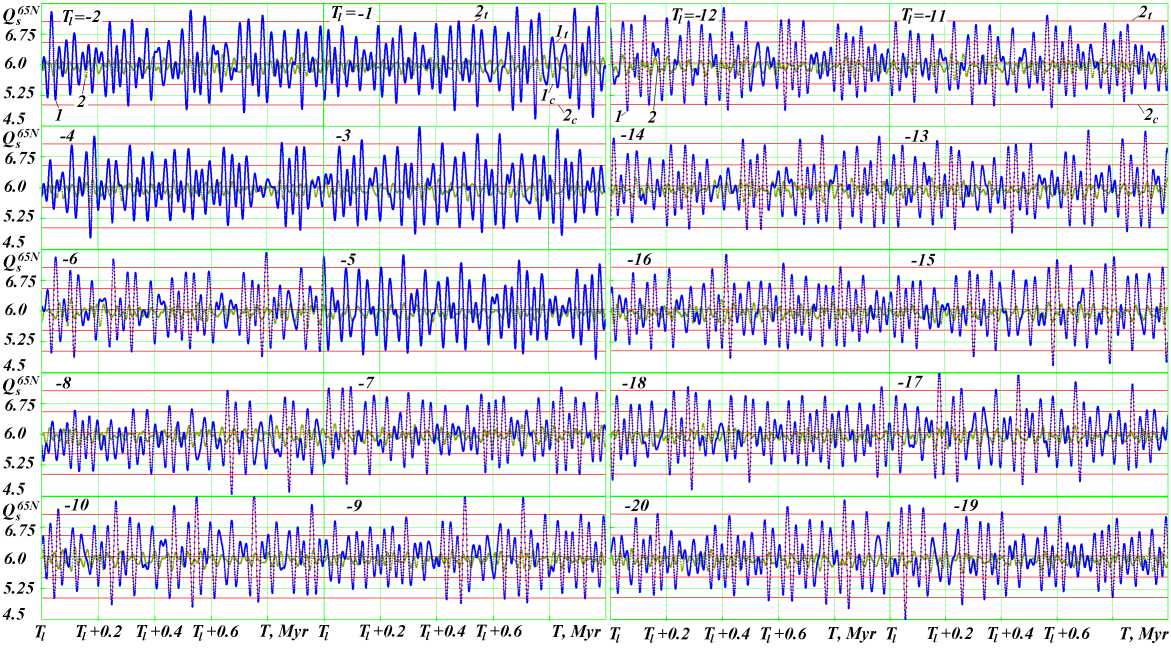
Fig.18. The evolution of summer insolation Q s ^{65 N} for 20 Ma in the form of 20 graphs for 1 million years (line 1 ); line 2 is summer insolation Q s ^{65 N} by Laskar et al. [24]; T l is the left reading of the time axis in million years, given in the left corner of each graph; 1t , 2t and 1c , 2c are the first and second boundaries of the warm and cold levels, respectively.

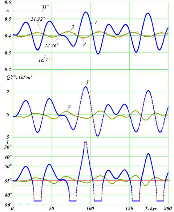
Fig.19. The evolution of the obliquity ε , as well as summer insolations Q s ^{65 N} and I for the span of 200 thousand years into the future.

Comparison of new results 1 with the results of previous theories on the example of the works by Laskar et al. [24] 2 and by Sharaf and Budnikova [25] 3 : obliquity ε is the angle of inclination in radians of the Earth's equator to the plane of its orbit; Q s ^{65 N} is insolation in GJ/m ² for the summer caloric half-year at the northern latitude of 65°; I is insolation in equivalent latitudes over the summer caloric half year at north latitude 65°. T is the time in a thousand years from December 30, 1949 [23].

The large and small values of Q s ^{65 N} (Fig. 17) are distributed unevenly in time. The large values of insolation I at equivalent latitudes indicate that at the latitude of 65° during those epochs there was more heat than nowadays at the equator. In other words, it is really very strong warming.

Simultaneously, the low values of I suggest that at the latitude of 65° the heat received by the Earth during the summer half-year was lesser than nowadays at the pole. Indeed, these are really ice ages.

The graphs (Fig. 18) show the changes in summer insolation Q s ^{65 N} during 20 million years in the form of 20 graphs, each graph representing a period of one million years. In the first graphs of the left panel, Q s ^{65 N} begins on the right for the first million years with the left countdown of time T l = -1 and, then, it continues beyond the second graphs T l = -2. The graphs end in the right bottom panel (-19) and (-20), i.e. with the 20th million of years.

The graphs show the unevenness of very strong warming and cooling of the climate. Here, one can find calm time intervals lasting one million years, when there were no strong climate fluctuations. This data is further evidence showing that, on the Earth, there were such climates that we do not know. Previously, all researchers were looking for the periodicity in the onset of glacial ices. Here, no such periodicity is observed. However, these changes occur with strict certainty and inevitability.

The lines 1 of the graphs (Fig. 19) show the variation of the obliquity ε, of insolations Qs65N and I over the summer half-year for the forthcoming 200 thousand years. Considering insolation I, one can see that very strong warming will occur in 90 thousand years. The same graphs for the future one million years (Fig. 20) show that there will be another strong warming that will occur in 900 thousand years. Thus, the next million years is characterized by smaller climate changes compared with the previous million years (Fig. 16).

0.6

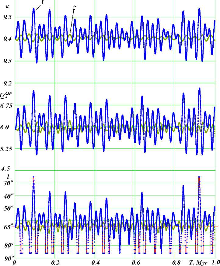
Fig. 20. The evolution of the obliquity ε , as well as summer insolations Q s ^{65 N} and I for the span of 1 million years into the future. Comparison of new results 1 with the results of previous theories 2 on the example of Laskar et al [24]. The interval between points is 200 years. The remaining designations see Fig. 19..

On the sectorial map of the Arctic (Fig. 21), the duration of polar nights is shown against the dark background, and the duration of polar days is shown against the yellow background in the three epochs: in the contemporary epoch 2025 year, 15.9 thousand years ago and 31.3 thousand years ago [26, 27].

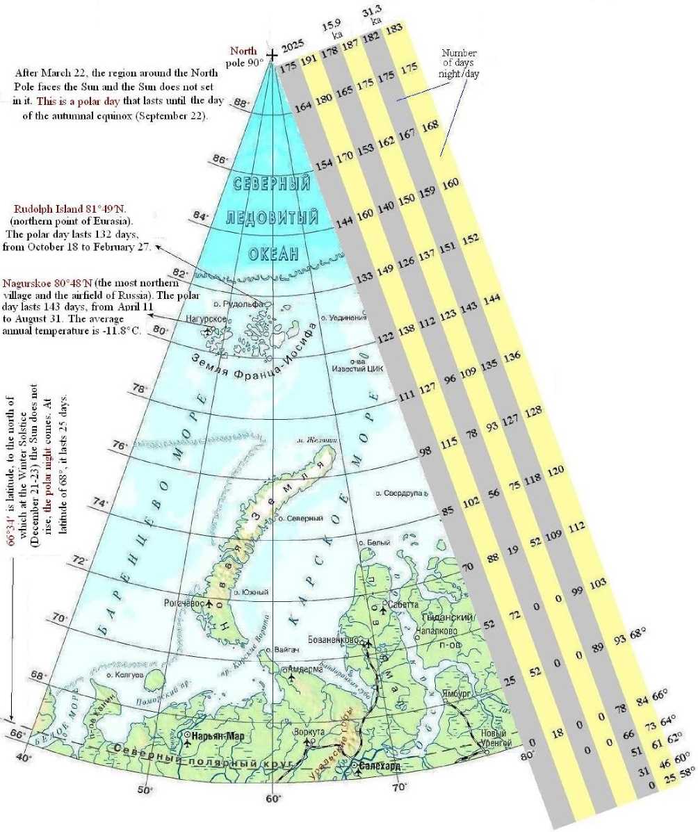
Fig.21. The duration of the polar night and the polar day in the Northern Hemisphere in three epochs: 2025, 15.9 and 31.3 thousand years ago. Latitudes from 90° to 66° are shown to the left of the picture, and from 68° to 58° are to the right of the picture.

In the contemporary epoch (2025), the polar night at the pole lasts 175 days, and the polar day – 191 days. At the latitude of 66 degrees, there are no polar nights anymore, and the polar day lasts 18 days. In the Sartan Ice Age, which occurred 15.9 thousand years ago, at the latitude of 70°, there are no longer polar days and nights. Next, in the extremely warm Karginsky period, which occurred 31.3 thousand years ago, at the latitude of 58°, the polar day lasts 25 days. The 58° is almost the latitude of Tyumen. That is, in an extremely warm period, here in Tyumen, as today at the Arctic Circle, the polar day lasts almost a month, and a short distance to the north we have a polar night. These data are further evidence for the Earth's climates which we do not know.

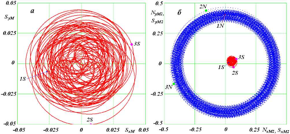
In the left graph (Fig. 22), the red line shows the motion of the orbit’s axis S over past 5 million years. The graph is the projection of the axis onto the plane normal to the precession vector MM (Fig. 13). The blue line on the right (Fig. 22) shows the precession of the axis of Earth rotation N projected onto the plane normal to the precession axis M2. On the same plane, the red line is the projection of the orbit’s axis S . The angles ε between the axes N and S in the corresponding epochs vary in proportion to the distances 1N-1S, 2N-2S, 3N-3S.

The presented data on the variation of insolation are due to the large fluctuations of the angle ε . Those fluctuations seven to eight times exceed the range of oscillations of this angle in the works by previous authors. These exceedances are due to the structure of the precession of the Earth orbit’s axis and the axis of Earth’s rotation revealed in the present study.

——

——

Fig.22. Projections of the precession trajectories of the Earth's orbit axis S (a) and its axis of rotation N (b) for 5 Myr on a plane perpendicular to ^—              — the vectors M and M , respectively. The positions of the axes at time points and angles between them: 1S and 1N for t = 0 kyr, ε = 23.443°; 2S and

2 N for T = -0.2326 Myr, ε = 30.778°; 3 S and 3 N for T = -2.6582 Myr, ε = 32.680° [2].

• IV.    Conclusions

Let us return to the problems posed at the beginning of the paper (Fig. 1). Then, 20 years ago, I thought: this is how one has to proceed with the work on the five stages. In those times, I would feel happy if I could accomplish at least the first three stages. Today, however, I see that I have all the five stages completed. The cause of the longterm climate fluctuations on the Earth is the interactions between bodies in the Solar system. These interactions lead to the fluctuations of the solar heat falling onto the Earth. The minima and maxima of this heat were identified with high accuracy: over 200 thousand years, accurate to several minutes, and over 100 million years, accurate to several days. These fluctuations are manifested in marine and continental sediments, in the form of relief, and the changes observed in the plant and animal world, including humans. Today the researchers, which work in these areas, that is geologists, geographers, geocryologists, biologists, historians and, even philosophers, face the problem of identifying those manifestations and correlating them to the extremes of insolation. As a result, we will get accurate and consistent knowledge about the past of our planet.

Acknowledgment

The materials of this work were obtained as a result of research at the Institute of Earth's Cryosphere, Tyumen SC of SB RAS, Federal Research Center for three decades, and in recent years, the research has been carried out under the project IX.135.2.4.

The results are based on the solution of the problems about the orbital and rotational motions obtained on supercomputers of the share use center at the Siberian Supercomputer Center, Institute of Computational Mathematics and Mathematical Geophysics SB RAS, Novosibirsk, Russia.