Conditions on Structural Controllability of Nonlinear Systems: Polynomial Method

Published Online April 2011 in MECS

• I.    I NTRODUCTION

  The structural property of systems presents the effect or action of parameters to systems. In 1974 Lin [1] presented a structured matrix, whose members are either constant zeros or independent non-zeros, i.e. non-zero members are independent parameters, to explore structural controllability of SISO linear systems. Shields etc. [2] used the structured matrix researched the structural controllability of MIMO systems. Willems [3] introduced a kind of matrix whose members are one order polynomial in parameters to investigate structural controllability of linear systems. Yamada etc. [4] presented a kind of column structured matrix, in which members of each column contain the same parameter, but different columns contain different parameters. Murota [5] defined and researched the so-called mixed matrix M = Q + T , where non-zero members in T are algebraically independent to those of Q over field K . Lu etc. [6,7] presented the rational function matrix with multiparameters description to coefficient matrices of systems and electrical networks and researched the structural properties over the field of rational function matrix with multi-parameters. For nonlinear systems, Fradellos etc. [8] used the term “structural controllability” to describe the property that if there is perturbation the nonlinear system is still controllable. He did not concern the parameters effects to nonlinear systems.

The conception of transfer function is just considered to belong to linear systems for long time. Of course, it plays an important role on analysis and syntheses. Until Zheng and Cao [9] introduced the transfer function to nonlinear systems, more researchers accept the fact that nonlinear systems can also have their transfer functions. Zheng etc. [10] explored the controllability of nonlinear systems using transfer function. Halas and Kotta [11] use this method to discrete time nonlinear systems. Halas [12]

researches the nonlinear time-delay systems using transfer function.

In this paper parameter space is introduced to nonlinear systems and structural controllability of nonlinear systems is obtained by transfer function. The rest paper is organized as follow: in section 2 some basic terms and mathematic knowledge are recalled; in section 3 the main result of this paper is given, i.e. the conditions of structural controllability of nonlinear systems ; in section 4 an example are used to illustrate the application of these conditions.

• II.    PRELIMINARIES

• A.    Parameter Space and Structural Controllability of Linear Systems in Frequency Domain [6,7]

Consider linear systems with the form

& = Ax + Bu (1) where state vector x e R" , input vector u e R m , A and B are matrices with proper dimension. Let z = ( z 1 ,L z q ) e R q be the parameter vector in this system. R^q is called the definition domain of z or parameter space. Let F ( z ) denote the field of all rational functions with real coefficients in q parameters z 1 ,L z q . F ( z )[ 2 ] denotes the polynomial ring in A with coefficients in members over F ( z ) .

Definition 2.1 : If each member of matrix M is a member over F ( z ) , then the matrix M is said to be a rational matrix or a matrix over F ( z ) . If all the matrices of systems are consider to be RFM, then the systems is said to be a rational function systems with multiparameters z or a systems over F ( z ) .

Now consider a systems over F(z) with the form x = Ax + Bu y = Cx + Du

where A, B, C and D are matrices over F(z) . Then its transfer function matrix can be denoted by

G ( s ) = C ( sI - A )^{- 1} B + D =

U ( s ) det( sI - A )

Q ( s ) U ^* ( s ) P ( s )

where P ( s ) = det( sI - A ) ∈ F ( z )[ s ] , U ( s ) = Q ( s ) U ^* ( s ) is a matrix over ring F ( z )[ s ] , Q ( s ) ∈ F ( z )[ s ] is the greatest common divisor of all members of U ( s ) .

Theorem 2.1 : If P ( s ) and Q ( s ) are co-prime, then system (2) is structural controllable, i.e. controllable over F ( z ).

Theorem 2.2 : If system (2) is SISO, then the system is structural controllable if, and only if, P ( s ) and Q ( s ) are co-prime.

Now two theorems about structural controllability of linear systems are given above. But our interest is how to extent these theorems to nonlinear systems analysis, so some mathematic knowledge is recalled follow.

• B.    Pseudo-derivations and Skew Polynomials

In this paper the nonlinear system considered is as follow

• & = f ( x , ^u )                    (3)

y = g ( x , u )

where f and g are meromorphic functions. x ∈ R ⁿ , u ∈ R ^m , y ∈ R^p .

Let K denote the field of meromorphic functions with the form F { x , u ^{( k )} , k ≥ 0} . Then the field K is endowed with a differential structure. Define a derivative operator δ over K , then

Sxi = x = f (x, u), i = 1,L, n gu j) = u (k+1), k > 0, j = 1,L, m

δF(x,u(k))= n ∂Fδx + m ∂F δu(k) ,         ∑i=1 ∂xi i ∑j=1 ∂u(jk) j k≥0

Generally, we use Su = U , u ⁽²⁾ = & . In order to handle theoretic properties of a system (3), we define a vector space ε of 1-form spanned over K by differentials of members of K with the form

ε = span{d ξξ ∈ K } .

Then each member of ε is a vector which can be denoted by v = ∑ a_i d ξ_i where a_i ∈ K . Again use the derivative operator δ on vector space, then the vector space is also endowed with differential structure, i.e. Sv = i&= ^ [ S ( a i^i + a , d( S^ )].

We know that in the expression of transfer function, the numerator and denominator are two polynomials in s . so the skew polynomial which can act as derivative operator should be introduced first.

Let K be a field, σ: K → K is a injective endomorphism mapping over K. A mapping δ: K → K is called pseudo-derivation if it satisfy δ(a+b)=δ(a)+δ(b) δ(ab) = σ(a)δ(b) + δ(a)b where a,b ∈ K . If σ = 1 , then the derivative law over K is the same as general derivative law.

The skew polynomial ring determined by δ and σ over K is a polynomial ring in s , and denoted by

K[s;σ, δ] , which is different from the general ring K[s] . The skew polynomial ring has the usual addition and non-commutative multiplication which is given by sa = as + &, a e K . Let V be the vector space over K, a mapping θ : V → V is called pseudo-linear if θ(u + v) = θ(u) + θ(v) θ(au) = σ(a)θ(u) + δ(a)u where a ∈ K , u,v ∈ V . For simple, we use recursively definition θku = θ(θk-1u) , k ≥ 1 , where θ0u = u . Then the skew polynomial can act on vector space and as operator. For the 1-form v in vector space ε, we have K[s;σ,δ]×V → V : (∑aisi)u = ∑aiθi(u)

Example 2.1 : Given a polynomial p ( s ) = s ² + x ₁ and a 1-form v = u d u , then p ( s ) ⋅ v = ( s ² + x ₁) u d u

= s ² u d u + x 1 u d u = s ( su )d u + x 1 u d u = s ( us + i& )d u + x 1 u d u

= us ² d u + 2 u&s d u + u d u + x 1 u d u = u d Як+ 2 г&Уг&+ u d u + x ₁ u d u C. Quotients of Skew Polynomial Ring

In section П -B, we define skew polynomials in transfer function. Now we should know the quotient law of two skew polynomials. There is no zero factor in skew polynomial ring K [ s ; σ , δ ] . Moreover, K [ s ; σ , δ ] satisfies the so-called Ore condition.

Lemma 2.1 (Ore condition): For all non-zero a ₁ , b ₁ ∈ K [ s ; σ , δ ] , there must exist non-zero a ₂, b ₂ ∈ K [ s ; σ , δ ] such that a ₂ b ₁ = b ₂ a ₁ .

By this condition we know that for each pair of members over K [ s ; σ , δ ] , there exist a common left multiple. By defining a quotient form as follow, ring K [ s ; σ , δ ] is embedded to a non-commutative quotient field [9-12].

a     - 1

= b ¹ a

b where a,b ∈ K,b ≠ 0 . The addition of two quotients is a a βa +βa denoted by 1 + 2 = 2 1    1 2 , where β b = βb ;

b 1 b 2        β 2 b 1

the multiplication of two quotients is denoted by ^{a 1} ⋅ ^{a 2} = ^{α 1 a 2} , where β a = αb .

^b 1 ^b 2     ^β 2 ^b 1              ^{2 1     1 2}

We denote the quotient field of skew polynomial by K s ; σ , δ .

Ш. STRUCTURAL CONTROLLABILITY OF NONLINEAR SYSTEMS

Now reconsider the nonlinear systems (3). This time we introduce parameter vector to the system. Then the nonlinear system containing parameters can be denoted as = f ( x , u , z )

(4) y = g ( x , u , z )

By differentiating (4), we have

d:& = A d x + B d u d y = C d r + D d u

where A = ( 5L ,L, f )  ,    в = ( 5L ,L, JL)

d x 1      dx n                d u 1      du m

C = ( 51 ,L, 5g. )    ,      D = ( 51 ,L, 2g )

dx1     dxn                      d u1     dum dx = (dx1,L , dxn)T , du = (du1,L , dum)T. Then we have

( si - A ) dx = Bdu dy = Cdx + Ddu

Finally we get

F ( s ) = dy = C ( si - A )^{- 1} B + D du

The equation (7) is said to be the transfer function (matrix) of nonlinear system (4).

Remark 3.1 : Expression F ( s ) in (7) is a polynomial over the quotient ring with coefficients in x , u and parameter z . Let K ( z ) denote the field of all functions in x , u and parameter z .

Definition 3.1 : A polynomial over the quotient ring with coefficients in x , u and parameter z is called a polynomial over quotient ring with multi-parameters, denoted by K z [ s ] .

The coefficient matrices A , B , C and D in equation (5) are matrices over K ( z ), so according to Definition 3.1 the transfer function (7) of nonlinear systems (4) is a polynomial over K z [ s ] .

Here we will give another definition about controllability of nonlinear systems form the view point of differential algebra.

Definition 3.2 : System (4) is said to be structural controllable if there exist no functions h : R ^{l + 1} ^ R and

w : R % ' ¹ x R^{m + 1} ^ R over F [ s , z ], such that

J h ( w , w L , w ^{( l} ) ) = 0

[ w = w ( y , y L , y ⁽%) , u , u ,L , u ⁽ m ) )

where l > 1, % + l = n , m % + l = m .

The map relation w in Definition is said to be autonomous variable, and the function h is called the autonomous function, so Definition 3.2 can be stated in another way: system (4) is said to be structural controllable if there exist no autonomous variable w and autonomous function h such that equation (8) holds.

Theorem 3.1 : Nonlinear system (4) is said to be structural controllable if the numerator and denominator of its transfer function has no common left divisor.

Proof: Let the transfer function (7) be denoted as follows dy = Qs!               (9)

du   P ( s )

Clearly, P ( s ), Q ( s ) e K ( z ). According to (9), we have P ( s ) dy - Q ( 5 ) du = 0.

On the contrary, suppose that there exists common left divisor R(s) e K(z), then R(s)(P*(s)dy - Q*(5)du) = 0, where deg P(s) = n , deg Q(s) = m , deg R(s) = l > 1 , then deg P*(s) = n -1 , deg Q*(s) = m -1 . Let R (s) = hlsl + hl-1 sl-1L + h0 , where hl ^ 0 , hie K (z) , i = 0,L , l . Let w = (P*(s)dy - Q*(5)du) e D1 , where D1 = span{dy1, duj\i = 0,L , n -1; j = 0,L ,m -1} . Then R(s)w = 0 , that is,

l

^ hw= 0 (10) i = 0

For equation (10), we know that it is just the autonomous function h , and w = ( P * ( s ) dy - Q * ( 5 ) du ) is the autonomous variable.

According to Definition 3.2 we know that the nonlinear system is not structural controllable. This is a contradiction. So for nonlinear system (4), it is structural controllable if the numerator and denominator of its transfer function has no common left divisor.

Now we will give another Theorem on structural controllability for SISO nonlinear systems.

Theorem 3.2 : For the SISO nonlinear system, it is structural controllable if and only if the numerator and denominator of its transfer function has no common left divisor.

Proof : By the above Theorem 3.1, the sufficiency of this Theorem is true, so we just prove the necessity.

On the contrary again, we assume that the SISO nonlinear system is not structural controllable, then there must exist autonomous variable w and autonomous function h such that equation (8) holds.

Now we can differentiate w and h with respect to their arguments respectively, and we get

% dw = Ё j=0

m dy^{(j )} + S k = 0

d w d y^(j )

d w дй ^ ¹^

dh dw(i)

l dh = ^

i = 0

_du ( k )

dw ^{( i )} = 0

Let dh = R (s) dw, dw = P (s) dy + Q (s) du, where R(s) = ^^whysi e K^[s],

%

P(s) = Z ^TFsj e K(z)[s ]                           , j=0 dy

Q ( s ) = 6-^ w-s k e K(z )[ s ]. £ 0 d u ^{( 11}

Now by the equation (11) we can get the relation

R ( s )( P ( s ) dy + Q ( s ) du ) = 0           (12)

From equation (10) we know that l > 1, % + 1 = n , Z m + 1 = m . Then equation (12) is just the transfer function of (4), and the polynomial R ( s ) is the left common divisor. So this is a contradiction, that is, if a SISO nonlinear system is structurally controllable then the numerator and denominator of its transfer function has no common left divisor.

Thus the whole Theorem is proved.

• IV .    STRUCTURAL CONTROLLABILITY OF C OMPOSITE

SYSTEMS

Polynomial method used in this paper has another advantage that it is convenient to explore composite nonlinear systems. In this section we will study the structural controllability of composite nonlinear systems.

For composite nonlinear systems, there are also three basic types, which are tandem, parallel and feedback composite systems. Here we will constrain ourselves to tandem and parallel systems.

Consider two nonlinear systems described by (4):

2 1 , its transfer function is denoted as

G 1 ( s )= ^{dy 1} = ^{B 1 ( s )}

du ₁     A ₁ ( s )

2 2 , its transfer function is denoted as

G 2 ( s )= ^{dy 2} = ^{B 2 ( s )} du ₂    A ₂ ( s )

Then the transfer function of tandem system 2 12 shown in Fig 4.1 (note: the order of subscript denotes the signal flowing from 2 1 to 2 2 and du 2 = dy₁ ) can be denoted as:

dy 2 B 2 ( s ) B 1 ( s )

G(s) =    = g du1    A2(s) A1(s)

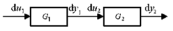
Fig. 4.1 tandem system

Clearly, G1(s), G2(s), G(s) ∈ K z [s] , A1(s), A2(s) , B1(s) and B2 (s) ∈ K(z) . Then for equation (15) the non- commutative multiplication is followed as

_{G ( s ) =} B 2 ( s )g B 1 ( s ) ₌ α ( s ) B 1 ( s )

A ₂( s ) A ₁( s )    β ( s ) A ₂( s )

According to Lemma 2.1, we have

β ( s ) B 2 ( s ) = α ( s ) A 1 ( s ) (17)

Proposition 4.1 : The composite nonlinear system 2 12 is structural controllable if its subsystems 2 1 and 2 2 are structural controllable and polynomials α ( s ) B ₁ ( s ) and β ( s ) A ₂ ( s ) in (16) have no common left divisor over the field of K ( z ) .

Remark 4.1 : Because the different composite manner and non-commutation, for the composite system 2 21 its transfer function is different from that of 2 12 . Then the following Lemma is immediate:

Lemma 4.1 : The composite nonlinear system consisting of two subsystems is said to be structural controllable if its subsystems are structural controllable and the numerator and denominator of transfer function of composite system have no common left divisor over K ( z ).

For the parallel composite system shown in Fig 4.2, we also consider the subsystems (13) and (14), then the transfer function of parallel composite system can be denoted as dy   B1(s) B2(s)

G (s) =   =      + p du   A1 (s) A2 (s)

Similarly, G ₁( s ), G ₂( s ), G_p ( s ) ∈ K z [ s ] , A ₁( s ), A ₂( s ) , B ₁( s ) and B ₂ ( s ) ∈ K ( z ) . For equation (18), the non-commutative addition is followed as:

B 1 ( s ) B 2 ( s ) β 1 ( s ) B 1 ( s ) + β 2 ( s ) B 2 ( s )

G„ ( ⁵ ) =--+--=------------------------ (19)

^p       A 1 ( s ) A 2 ( s )            β 1 ( s ) A 1 ( s )

According to Lemma 2.1 we have

β 1 ( s ) A 1 ( s ) = β 2 ( s ) A 2 ( s )

Then for the parallel composite system, the following proposition is true.

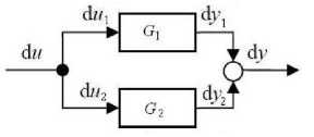
Fig. 4.2 parallel system

Proposition 4.2 : The parallel composite system with two subsystems is said to be structural controllable if its subsystems are structural controllable and the numerator and denominator of transfer function of parallel composite system have no common left divisor over K ( z ).

In view of practice parameters in each subsystems can be different, then let z ∈ R ^q in subsystems (13) and z ′ ∈ R ^{q ′} in subsystems (14) and R ^q I R ^{q ′} = Φ , where Φ denotes the empty set. Then for tandem composite system 2 12 , the following Theorem is true:

Theorem 4.1 : A physical tandem composite nonlinear system is said to be structural controllable if its subsystems are structural controllable and the numerator and denominator of transfer function of tandem composite system have no common left divisor over K [ s ; σ , δ ].

Proof :  By  the  assumption it is  known  that

A ₂( s ), B ₂( s ) ∈ K ( z ′) , A ₁( s ), B ₁( s ) ∈ K ( z ) , then by equation  (17)  and  Lemma 2.1 it is known  that

0 ≠ β(s) ∈ K(z) , 0 ≠ α(s) ∈ K(z′) . For the noncommutation, it is necessary to consider whether α(s) and β(s) have common left divisor or not. Since the polynomial α(s) ∈ K(z′) , if it can be decomposed then there exist at least one root belonging to the field of K( z ′ ) and at the same time not belonging to K(z). Similarly, for polynomial β(s) ∈ K(z) , if it can be decomposed then there exist at least one root belonging to the field of K(z) and at the same time not belonging to K( z ′ ). Because K ⊂ K(z) and K ⊂ K( z′ ), then only if α(s) and β(s) have the left divisor over K[s;σ, δ] (i.e., the root of left divisor over K) there would be existence elimination. So for two subsystems with different parameters respectively, the tandem composite system is structural controllable if its subsystems are structural controllable and the numerator and denominator of transfer function of tandem composite system have no common left divisor over K[s; ст, 5].

• V.    APPLICATIONS

In this section, we give some examples to show the applications of above Theorems.

Example 5.1 : First consider a simple nonlinear passive RLC network showed in Fig 5.1, where the nonlinear resistance voltage is u_R = ki ² , k is a gain, the inductance is L , the capacitance is C . suppose that the input voltage is u_i and the output voltage is u_o . Then by KVL , we have

F ( s ) =----:------:-----, which is in the form of input

LCs ² + 2 kC ² ys +1

and output. Clearly, the numerator and denominator of this transfer function has no common left divisor, so this nonlinear system is structural controllable, this is , when the parameter z takes values in parameter space R ³ , this nonlinear system is controllable. This result is the same as that in [13], where we use differential geometry to handle the structural controllability.

Example 5.2 : Now we consider a composite nonlinear system as another example.

Consider two subsystems as follow:

I 0/ = u * - ax /         I X 2 = au 2

z * ^: S                   Z 2 ^: S

[ У 1 = x i                 [ У 2 = ^x 2

d i 1             2

L --+ i d t + ki d t C

= u

S

_ uo = C J 1 dt

By calculation we have G. ( s ) =---- —r- and

12 s + 3 ay 1

Let x1 = i, x2 = uo, u = ui, y = uo , then we can get the state space description as follow x = yCu-x2 -kx2)

^S x = C ^x 1                       (20)

3 au ²

G 2 ( s ) =---- . We consider the tandem

s system J12, and then transfer function is

dy ₂    B ₂ ( s ) B ₁ ( s )   3 au ₂ ²

composite

s + 3 ay *

У = x 2

Because the signal flows from J 1 to J ₂, du ₂ = dy ₁ . So equation (21) can be written to

G (s) = 3ay2g-^-r s s + 3 ay1

then

where the parameter z = ( L , C , k ) e R ³ .

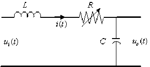
Fig 5.1 a nonlinear passive RLC network

( 2 k

^^^^^^»

According to non-commutative multiplication in Lemma 2.1, equation (22) changes to

G ( s )=     ^{3 ay} 2₂

( s + 3 ay *² ) s

By differential to (20), we get

A =

L

x ₁

B =

I 0 J

, C = (0 1) . Then

I C

L

Then the tandem composite system J 12 is structural controllable.

Let us consider the composite system J21, the transfer function is

G ,₍ s ) = j y . = B 1 ( ^s ) g B , ( ^s ) =     ¹ 2 g ^{3 a}« ;      (24)

du ₂    A 1 ( s ) A ₂ ( s ) s + 3 ay 1²    s

In this case the signal flows from J 2 to J 1 , then du ₁ = dy ₂ . According to non-commutative multiplication

equation (24) changes to

(sI - A)-1

_r z , 2 kx. A i / ^{Ls ( s +} 1/L )^-/ C

C ( s + ² kx /) s + U

\         / L / L

______________1______________'

Ls ( s ■ ² A) ^- Ус

C ( s - ² kxL )

C ( s + ² kx¹/ ) s + U

/ L / L 7

G ‘( s )

3 au ₂ ²

s ( s + 3 ay 2 )

Clearly, the tandem composite system J 21 is structural controllable.

Now let us consider these two subsystems with different parameters as follow:

So by calculation

the transfer

function F ( s ) = C ( si - A ) ¹ B , we get

I ix1 = u 1 - ax 3         I xx 2 = bu 2

^J a ^: S                  ^J b ^: S

[ y 1 = x 1                 [ y 2 = ^x 2

F ( s ) =

LCs ² + 2 kCx 1 s +1

Let us consider the tandem system J ab only, the

transfer function is

Since x ₁ = Cx &₂ = Cy & , the transfer function of this nonlinear system can be finally denoted to

G ab ( s ) =

dy ₂ du ₁

3 bu ²      1

-----g ^ 1 2

s   s + 3 ay ₁ ²

According to non-commutative multiplication equation (26) changes to

G (Ss ) = — '        PSs ) s

According to Lemma 2.1 it is known that в ( s ) ■ 3 bu 2 = a(s )( s + 3 ay^) , then we can make the polynomials a(s ) e K ( b ) and ^Ss ) e K S a ) • By

calculation we know that a ( s ) and в ( s ) are one-degree

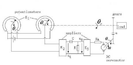
Fig 5.3 a servo control system

polynomials in s, so a ( s ) and в ( s ) have no common left divisor. For simple explanation, we can let polynomial a ( s ) = 1 be constant number, then

в(s ) e K ( a , b ), it is clear that transfer function G_ab ( s ) has no common left divisor. Of course G_ab ( s ) can not has common left divisor over K [ s ; o , 5 ] . So the tandem

system J ab is structural controllable.

Example 5.3 : In this example we consider a multiinput multi-output system containing two networks as shown in Fig 5.2.

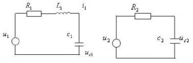
Fig 5.2 a multi-input multi-output system

The system has five physical parameters R ₁ , L ₁ , C ₁ ,

Neglect the nonlinearities of the motor and the gears. The system may be considered to be a composite system containing three subsystems J 1 with the input A O = O r - O_c and the output u_R , J₂ with the input u_R and output O_c , and J ₃ in the feedback path with the input O_c and the output O_c . Choose three state variables u_c , w , O as shown in Fig 5.3. Then

2 1 : U c = - a 0¹) u c + a 0¹) d 1 A O , u_R = - u c + d 1 A O , where

a 7 = -^, d = k,k ₂, a 7 d = YY, 0 _RC 1    1 2  0  1 _RC

Г O I Г 0

2 :      =

² V & 7 V ⁰

where

—

1 Y о I Г 0   I

<2) II I ⁺1          I ^U R ,

• a S) 7 V to 7  V b) 7

O c = S n ,0)

о to

R ₂ and C ₂ . The state equation of the system

X = AX + BU , y = CX , where

is

X =

A =

^ X 1 A

x ₂

V x 3 7

Г--

L

C

^^^^^e

u c 1

V u c 2 7

L 1

V

I U I

, U = | ¹ I, Y =

V u 2 7

i ₁

x ₁

I

, B =

Г 1

L 1 0

u c 1

x ₂

, C =

10 1 0

• S2)    frnR-a ^{+ k} b ^C m Z.S2)    ^k 3 ^C m

• a, =-----------------, b.   =--------.

• ¹         J m R a      ⁰     J m R a

2₃ : O_C = O_C

The parameters of J 1 and J 2 are obviously independent of each other. Let z ^S1) = S C , R , k 1 , k ₂) e R ^{4 and} z ⁽²⁾ = ^S J m , R a , f m , k b , ^C _m , k 3 , n ) ^{e R} 7 . ^J 3 ^{has no} physical parameters. Then the total system J has eleven parameters z = S z ⁽¹⁾, z ⁽²⁾) e R ¹¹ . Clearly J ₃ is structural controllable. Since

ТЕ

2 2 7

V

IV 2^2 7

G 1 S s ) = ^1^, G 2 S s ) = s + a 0)

b0(2)n sSs + d1S2)) ’

The transfer function of the system is

S s +¹—) R 2 C 2

G S s ) =----

S s +

1¹ s

L ¹

V L 1 C

1 R 1

)[ s S s + 1 ) +     ]

R ₂ C ₂         L ₁     L ₁ C ₁

Since the numerator polynomial matrix and denominator polynomial have the common divisor S s + 7 R 2 C ₂) , the system is not structural controllable by Theorem 3.1.

Example 5.4 : Consider a servo control system as shown in Fig 5.3. O r and O_c are the input and output of the system, respectively.

The numerator polynomial and denominator polynomial of G S s ) S i = 1,2) have no common divisor,

that is, J 1 and J 2 are structural controllable. Since the initial conditions of energy storage elements of 2 j S i = 1,2) are independent. Thus structural controllability of the tandem composite system J₁₂ are only dependent on the zeros and poles at origin [14], but P ₂S0) = 6 1 S0) = 0 , then J ₁₂ is not structural controllable. So J is not structural controllable.

^. CONCLUSIONS

In this thesis the new field K ( z ) and ring K z [ s ] , which contain the parameter vector z , are defined. The differential algebra and pseudo-linear algebra are used to obtain the transfer function of nonlinear system. Parameter space is introduced to the analysis of nonlinear

Systems, and conditions of structural controllability in frequency are presented. Examples are used to testify the conditions. Composite nonlinear systems are researched and structural conditions on controllability of tandem and parallel systems are obtaind. The transfer function method has advantages on researching composite nonlinear systems, and maybe we can get the globle properties of nonlinear systems which are interested to us.

A CKNOWLEDGMENT

The author wishes to thank professor Lu Kai-sheng. His some useful suggestion helps me improving this paper. The author also wishes to give his thanks to anonymous reviewers. This work was supported in part by National Nature Science Foundation of China under grant: No. 50177024.