Conforming identification of the fundamental matrix in the image matching problem

The task of identification is to construct an optimal model of an object (system) from the results of observations of the input and output data. Often the identification of an object should be performed using an extremely small number of measurements. This may be due to the requirement of efficiency, excessive cost or the impossibility to obtain a large number of measurements, etc.

In this case, the so-called conforming identification method (CIM), which does not require a priori assumptions about the distribution of measurement errors, can be applied. This method was considered in papers [1, 2] discussing the task of identification of a controlled object. An important feature of this method is its robustness to gross errors such as failures. In the case of normal observation errors, the results usually coincide with the ones obtained by least square method (LSM) and least absolute deviations method (LADM) procedures.

The high accuracy and reliability of the method in this case is provided by using a large number of subsystems, formed by various combinations of the rows of the initial system. However, because of this, the method has a high computational complexity and memory cost. Thus, it becomes necessary to develop a parallel algorithm to be implemented on a multiprocessor system.

In paper [3] authors propose a method of conforming identification of the fundamental matrix from set of corresponding points. In this paper we study the accuracy and reliability of the conforming identification method in comparison with other commonly used methods.

K 1 = K 2 = K =

f 0 0

0 u ₀ f v ₀ 01

where f is a focal length of cameras, ( u 0 , v 0 ) are coordinates of the main points of the cameras in the coordinate systems associated with the cameras.

Let M be a point in the global coordinate system. The coordinate vector of point M in the global coordinate system is related to the coordinate vectors of this point m 1 and m 2 in the coordinate systems of the first and second cameras by the equation [4]:

m1 = P1M, m2 = P2M, where the projection matrices are defined as

P i = K i [ R i • t i ] ,

P ₂ = K ₂ [ R 2 : t 2 ] .

Here R 1 , R 2 are the 3×3 matrices describing the rotation of the coordinate systems of the first and second cameras relative to the global one, and t 1 = [ t 1, x , t 1, y , t 1, z ] ^T , t 2 = [ t 2, x , t 2, y , t 2, z ] ^T are coordinates of the origin of the global coordinate system in the coordinate systems of the first and second cameras, respectively.

The matrix R is formed as

R = R X R Y RZ , where

	( 1	0	0	)
R x =	0	cos ( a )	± sin ( a )
	v 0 + sin ( a ) л cos ( e )    0		cos ( a ) ± sin ( p ) Л	7
R Y "	01 v + sin ( p ) 0		0 cos ( P ) ;

R

Z

' cos (y)   ± sin (y) 0"

+ sin ⁽Y )    cos ⁽Y )    0

v 0           0       1 ,

The corresponding points on two images are related by a fundamental matrix [4]. For points whose coordinates are given by 3×1 - vectors m 1 = [ u 1 , v 1 , 1] ^T and m 2 = [ u 2 , v 2 ,1 ] , the condition

• m , T F m 2 = 0

is satisfied, where

F 11	F 12	F 13
F 21	F 22	F 23
F 31	F 32	F 33

The equation for calculating the fundamental matrix has the form:

F = K-T [t ]x RK-1, where [t]× is constructed as

[ t L = 1 3

. - t 2

- t 3

t ₁

t ₂

- t 1

.

For N pairs ( N ≥ 8) of corresponding points, assuming that F 33 = 1, a system of linear equations can be formed to estimate the vector c of the desired fundamental matrix values:

с     [ c 1 , c 2 , ..., ^c 8 ]

= [F11, F12, F13, F21, F22, F23, F31, F32 ] , where

'''

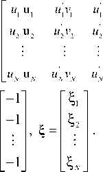
v ₁ u ₁ v ₁ v ₁ v ₁ u ₁ v ₁

'''

v ₂ u ₂ v ₂ v ₂ v ₂ u ₂ v ₂

v ^' u     v ^' v     v ^'      u v

NN NN N N N

^ are errors related with inaccurate calculation of the coordinates of the corresponding points.

Estimate с ˆ of vector c can be obtained by solving the system (2) using the LSM, the LADM, RANSAC [5], or conforming identification. The number of observations, on which the system (2) is formed, is extremely small, therefore, we apply the conforming identification method.

• 2.    Formulation of conforming identification problem

We consider the problem of estimating the vector с of linear model parameters:

y = Xc + ^ ,

where y and X are N×1-vector and N×M - matrix observed in the experiment, and ^ = [^i, £2,..., ^n] T is Nx1- vector of unknown errors. The matrix X is composed of rows xi, i = 1, N. The task of identification is to calculate vector of estimates cˆ using observations y and X.

If there is no a priori error information, then the leastsquares method is usually used:

c = [ X T X ]^{- 1} X T y .

It is known that LSM estimates are unbiased and effective under the usual assumptions. However, with a small number of observations, these assumptions prove to be unreliable because of the insufficient statistical stability of probabilistic characteristics. The method of conforming identification is based on the assumption that the solutions obtained on the subsystems that are most free of noise will be closer to each other (i.e., conformed), and the task is to determine such a subsystem. Here is a brief description of the identification algorithm based on the principle of conformity of estimates.

A certain set of subsystems of small dimension is "extracted" from the initial system (3):

y k = X k c k + ^ k , k = 1,2,..., K .                       (4)

Each subsystem (4) contains the rows of the initial system (3). Let us further refer to these subsystems as lower-level subsystems. In this case, the set of lower-level subsystems contains subsystems with square M × M -matrices X k . By calculating an estimate c ˆ _k from available observations X k , y k for each subsystem (4), we can obtain C_N^M possible estimates on lower-level subsystems.

Similarly, it is possible to form a set of C_N^M higher-level subsystems of P × N dimension:

y 1 = X 1 c 1 + § 1 , l = 1,2,..., L ,                           (5)

Each l^th higher-level subsystem (5) contains a set of lower-level subsystems (4), on which the corresponding set 0 ( l ) of estimates .. is calculated:

0 ( l ) = { c _l , _k e 0 ( l ) } l = 1 L , k = 1, K .

To characterize the conformity of sets 0 ( l ), a function of mutual proximity of the estimates is introduced:

K ₂

W ( l ) = Ё ( c l , i - c l . / ) ,                                (6)

i, j=1, i * j where cl,i, cl,j, l = 1, L, i = 1, K, j = 1, K are the estimates obtained on lower-level subsystems contained in the lth higher-level subsystem. Indices i and j in the right side of the expression (6) take all possible pairs of values. The set 0(l) of estimates clk, k = 1, K, K = CpM with minimum value of W(l) is called the most conformed one.

The hypothesis is that the most conformed subsystem is the most noise-free, so the task is to find the index l ˆ of the higher-level subsystem:

W (/) = min W ( l ), l = 17 L , L = C^P_N .

At the l ^th higher-level subsystem, we can either calculate an estimate or a "cloud" of estimates [2].

Admittedly, the implementation of the described conforming identification algorithm requires large computational resources. So computing time for identification problem with parameters N = 10, M =5, P = 9 is 0,01 seconds and computing time for identification problem with parameters N = 18, M = 9, P = 16 is 793.530322 seconds. This is due to the lack of a priori information and a small number of observations. That is why it becomes necessary to use an efficient parallel algorithm to decrease the computation time.

3.    Parallel algorithm of conforming identification

In paper [6] a parallel algorithm of conforming identification was considered. Sets of higher-level subsystems were formed on different processors. Subsystems indices are formed sequentially because it is necessary to form all possible indexes, which leads to the downtime of the processors. It is worth noting that the indices of the subsystems of the subsystems of the upper and lower levels can be formed once. It will eliminate the downtime of the processors in further calculations of the solutions.

Fig. 1 shows the general block diagram of the proposed algorithm and detailed diagrams of the algorithm stages, where Fig. 1 a shows general block diagram, Fig. 1 b demonstrates data loading and subsystem generation, Fig. 1 c shows the calculation of the higher-level subsystem with the least conformity coefficient for each thread, and Fig. 1 d shows the selection of the higher-level subsystem with the least conformity coefficient and calculation of the solution.

Because of the need to combine all the results of calculations, the master-slave communication topology and MPI are used.

For the above algorithm, the speedup and efficiency characteristics were calculated by solving the identification problem with parameters N = 18, M =9, P = 16. The results are shown in Table 1. The calculations were performed on a supercomputer “Sergei Korolev”. One node with two processors, which have 4 cores each, was used.

The data in Table 1 shows that constructed parallel algorithm is well scalable. Its execution time decreases almost linearly proportionally to the number of threads used. This algorithm is quite efficient because the calculation is evenly distributed among the threads. With the increase in the dimension of the original system (the number N of rows), the execution time of the program is significantly increased.

Table 1. Speedup and efficiency of the parallel algorithm

Number of threads	Execution time (sec.)	Speedup	Efficiency
1	793.530322	1.000000	1.000000
2	399.019544	1.988700	0.994350
3	264.601322	2.998966	0.999655
4	202.061476	3.927173	0.981793
5	170.967832	4.641401	0.928280
6	145.024123	5.471713	0.911952
7	139.921319	5.671261	0.810180
8	103.603291	7.659316	0.957414

4.    Experimental study of accuracy and reliability

When modeling the initial data, the following parameters are used:

^ a = 0 ^

^{e 0}

( Y = 0 J

R i =

	" 960	0	960 "		" 0
K = K 1 = K 2 =	0	540	960	t = , t1 =	0
	0	0	1 _		0

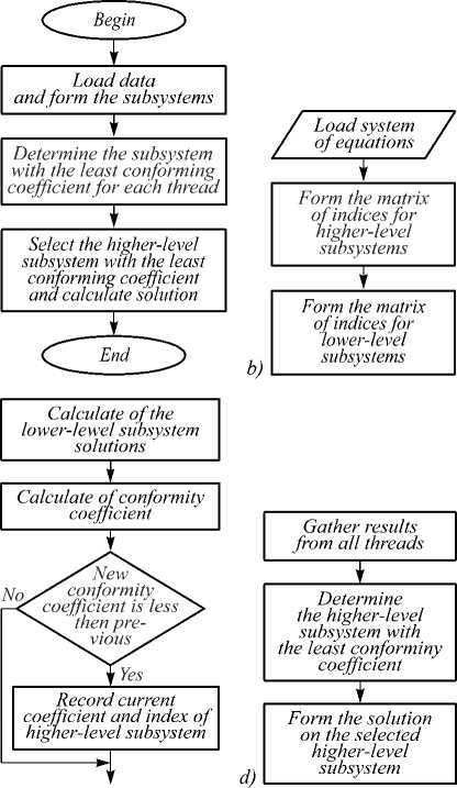
Fig. 1. Block diagram of the algorithm

When forming the elements of the matrix R 2 in (1), the angles a ? , p 2 , 7 2 are set in the interval [0 ° , 8 ° ]. Vector t 2 is specified as follows:

t 2 =

x

y

p cos( ^ )

P sin( v )

pe [5,6], фе [0,360], z e [-1,1].

z z

With the above mentioned parameters, 100 sets of points m 1 and m 2 are generated. In the formed sets of points Gaussian noise with SNR=70 and mean equal to zero is added. Then a random gross error is added. For each modeled set of corresponding points, a system of linear equations is formed. Next, estimates c ˆ of the fundamental matrix coefficients are calculated using the LSM, the LADM, and the conforming identification method. Each element of the resulting matrix F is normalised:

F = F / k , k = E F .

V i , j = 1

Table 2 gives an example of the obtained coefficients of fundamental matrices calculated using the LSM, the LADM, and the method of conforming identification (CIM).

Table 2. Calculated coefficients of fundamental matrices

Coefficients	LSM	LMM	CIM
F 11	-0.000000014	-0.0000000109	0.0000000117
F 12	0.0000002480	0.00000023645	0.00000122083
F 13	-0.0002013594	-0.0002574948	-0.0025098495
F 21	-0.0000000731	-0.0000000565	-0.0000008167
F 22	0.00000021004	0.00000021202	0.00000026023
F 23	-0.0037893080	-0.0038348863	-0.0055635209
F 31	-0.0001750568	-0.0000485521	0.00181021209
F 32	0.00287111864	0.00309045186	0.00477540238
F 33	0.99998935123	0.99998783697	0.99996833277

To determine the reliability of methods for each system, a set of 500 corresponding points m 1 and m 2 is generated. For each pai r of c orresponding points, distances to epipolar lines d_i , i =1,500 are calculated:

d = | l i 1 u ⁺ li 2 ^{V +} li 3 | ‘ V ^l' ' ^l'

where ( l i 1 , l i 2 , l i 3 ) are calculated as follows:

l = u • F , where l = [li 1, li2, li3]T, u = ^ui, vi ,1] . As a measure of the accuracy of the methods, values dk, k=1,100 are used. They are calculated by the formula:

K dk = к E d2i \ ,(7)

V K i=1)

where d ki is the distance from i^th test point to the epipolar line for k ^th set of points m 1 and m 2 , K = 500.

Table 3 shows the maximum and minimum values of d k for each method.

Table 3. Values of d k

	LSM	LADM	CIM
Maximum value	384.92	476.20	339.90
Minimum value	2.36	2.36	1.02

For a set of values d k calculated by formula (7), histograms are formed. Тhe interval of possible values is divided into 20 intervals A d , l = 1,20 and for each interval, the probabilities p) l for the values of the criterion d k e A d l are determined:

m pl= N E Nl- where N is total number of generated points, Nl is the number of points included in the lth interval of the histogram, m is the number of intervals of the histogram. The histograms and the estimated distribution function of the accuracy dk for each method are shown in Fig. 2.

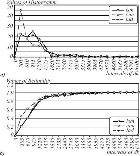
Fig. 2. Histograms of d k (a); Reliability graphs of accuracy (b)

The graphs in Fig. 2 show that the conforming identification method has higher accuracy and reliability in comparison with the LSM and LADM. In the problem of fundamental matrix identification, the least-squares solution will give a more accurate solution than the LADM.

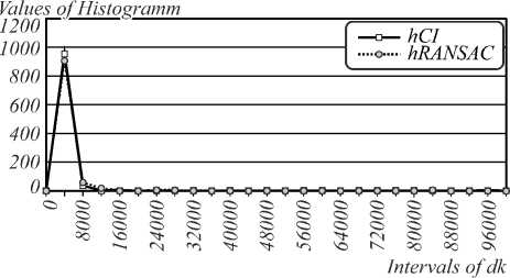
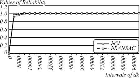
The study of accuracy and reliability of the CIM and RANSAC methods was also carried out. Fig. 3 shows a histogram of distances and distribution function of d k . for both methods.

The graphs in Fig. 3 demonstrate that the CIM slightly exceeds the RANSAC method in accuracy and reliability. Also, unlike RANSAC method, the conforming identification method does not require setting the threshold value and the number of iterations.

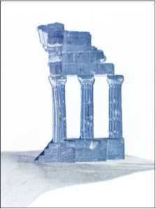
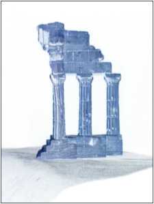
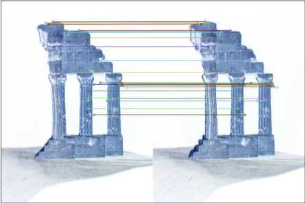
The algorithm was applied to real images form the set “Temple of the Diskouroi”. To find the feature points in the images the algorithm SURF [7] from OpenCV library was used. Figure 4 shows the selected images and the obtained corresponding points.

Using the selected feature points, we obtain a system of linear equations to which an extra gross error was added, and the fundamental matrix is further calculated. Similarly, for the generated test points the distance d i , and then parameter d were calculated. The conformity coefficients for the CIM and RANSAC equal 8803,506 and 12297,313, respectively.

Conclusion

Experimental studies demonstrate that for the problem of the fundamental matrix identification the method of conforming identification ensures a more accurate solution, and has a higher reliability as compared to the LSM and the LADM. The conforming identification method slightly exceeds the RANSAC method in terms of accuracy and reliability. Also, the CIM does not require setting the threshold value and the number of iterations.

а)

b)

Fig. 3. Histograms of d k (a); Reliability graphs of accuracy (b)

b)

c)

Fig. 4. Test images (a, b); selected feature points (c)