Cyclic analysis of extra heart sounds: gauss kernel based model

Published Online May 2018 in MECS DOI: 10.5815/ijigsp.2018.05.01

The analysis of cardiac signals by auscultation, based solely on human hearing, remains insufficient for a reliable diagnosis of heart diseases and for a clinician to obtain all qualitative and quantitative information about cardiac activity. This information such as the temporal location of the heart signals, the number of their internal components, their frequency content, the importance of diastolic breaths and systolic devices can be studied directly on the Phonocardiogram (PCG) signal by the use of signal processing techniques. PCG is an effective method for tracking the progress of the patient’s diseases. Auscultation has long been important for the heart diagnosis. Heart sounds heard by a stethoscope can be seen as mechanical instructions that indicate the functioning of the cardiac system. A PCG signal, in the healthy case, consists of two fundamental sounds s1 and s2 as shown in Fig. 1 which are derived from the mechanical functioning of the heart. The heartsounds1, corresponding to the beginning of the ventricular systole, is due to the closure of the atrio-ventricular valves. Where the heart sound s2, marking the end of the ventricular systole and signifying the onset of the diastole, corresponds to the closure of the aortic valve and the pulmonary valve. It is well known that s1 and s2 are defined as non-stationary signals, and are located in the low frequency range, approximately between 30 Hz and 75 Hz [5, 10, 14, 15, 17, 18]. A triple rhythm in diastole is called a gallop and results from the presence of a heart sound s3, s4 or both. In particular, the third heart sound s3 appears in early diastole, 120 to 180 ms after s2, whereas, the fourth heart sound s4 appears in presystolic portion of diastole. The frequency of s3 is between 30 and 50 Hz. s4 is low frequency with respect to s3 with frequency between 20 and 30 Hz. The frequencies can occur only under very precise conditions (Childhood or old age as signs of any pathology) [2, 11]. It should be noted that s3 and s4 have significantly smaller amplitudes and low frequencies with respect to the normal signals. An Extra Heart Sound (EHS) may not be a sign of disease. However, in some situations it is an important sign of disease, which, if detected early, could save lives. Unfortunately EHS cannot be correctly detected by ultrasound. Hence the need of EHS early detection approaches. Several studies have been interested in the analysis of PCG signals; however, most of them are based on the occurrence of time-frequency analysis or scale [6, 7, 8]. To the best of our knowledge, all these tools do not completely exploit the periodic behavior of PCG signals due to the functioning of the heart. As a matter of fact, the heartbeats are in the form of a series of repeated mechanical actions. The repetition is almost periodic. In other words, the vibration waves records are, in a sense, cyclostationary [1, 9, 12, 13, 16]. Hence, the need for mathematical models describing the functioning mechanism of the heart sounds is compulsory. This article aims to present a cyclostationary model for PCG signals with extra heart sounds. This model is extensively developed in order to evaluate to what extent it is adaptable to the heart functioning. The major motivation behind the new model is to introduce a framework for an accurate characterization of PCG signals with extra heart sounds and thereby an early detection of certain abnormal heart functions. For this reason, the EHS model and its theoretical development are systematically compared with the one of healthy PCG signal [17] in order to recognize the feature allowing the early identification. The key idea is the fact that cyclic statistics are not influenced by stationary additive noise. The choice of cyclic statistics is justified by the wide-sense cyclostationarity property of the proposed model as it is shown in section 3.

A stochastic signal x ( t ) of mean { x ( t )} and timevarying autocorrelation function R_x ( t , t ) = E{ x (t — t / 2) x *( t + t / 2) } , where the superscript * denotes complex conjugation, is said to be wide-sense cyclostationary with T 0 -period if both IE { x ( t )} and R_x (t , t ) are periodic over time t with T₀-period [3], i.e. E{ x ( t )} = E{ x ( t + T ) } for all t

R_x (t , t ) = R_x (t + T , t ) for all t, t. The time-varying autocorrelation function is, thus, periodic over t and can be expanded in Fourier series:

+^              j 2 n

Rx (t,t) = S Rn/To(t)e   T0  , where Rx/T0 (t)  is n=-m known as the cyclic autocorrelation function and is given n

1    To/2      ,    . - j2nV t by:    R—/To(t) =         Rr (t,t)e    T0 dt    ,where x               - T/2 x

T0   0

n / T , n gZ are the cyclic frequencies. The Fourier transforms the cyclic autocorrelation function with respect to the cyclic frequency α and gives rise to the spectral correlation density function:

S“ (f) =  +” R“ (t) e- j 2naTdT.

-да

This article is organized as follows: Section 2, describes the modeling of PCG signals. Section 3 is concerned with the analytical study of the proposed model, some simulation results are also presented in this section in order to confirm the theoretical analysis. Section 4 focuses on the validation of the computed cyclic statistics on synthetic and experimental PCG signals. Finally, Section 5 is dedicated to conclusions.

• II.    Modeling of PCG signals with Extra Heart Sounds

As mentioned in our previous work [17], the Gauss kernel, which is actually a Gaussian-damped sinusoidal wave, offers the possibility, through five adjustable parameters ( a_t , ^ , ц. , f and ^ ) , to definitely recreate the shape of any heart beat. The model of (1) makes use of two Gauss kernels to represent each heart sound s 1 and s 2 . Therefore, one normal heart beat of PCG signal can be modeled with four kernels as follows (Fig. 1):

^ a exp I- ⁽ t - ^^ )  | cos ( 2 n / ;^t - ^ , -)      ⁽¹⁾

i G [ 5 ± ; 5 ± ]           V       ² ^ i     )

Where

•   fi and 9i are respectively the frequency and the phase shift of the sinusoid terms.

at, ^, and ^ are respectively the amplitude, the center and the width which represent the parameters of the Gaussian terms.

± is a superscript indicating the two Gabor kernels which are used for modeling each heart sound, with

[ ⁵ ! ; ⁵ 2 ^] = ^{[ 5} 1 , ⁵ 1 ;

s ₂ , s ₂ ] .

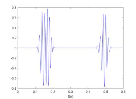
Fig.1.Example of healthy PCG signal for a single heart cycle of (1).

As a matter of fact, the signal model of (1) can be extended to take into account the presence of an EHS s 3 , s 4 or both (Fig. 2, (c, e, g)) as follows:

S a exp I ^-^ t T ^ i )" I ^cos ( 2 n ft ^- ^ ) ⁺ S q^ f exp I [ 5 ± ; 5 ± ]            V        ^{2 G} i )                                i g [ 5 ± ; 5 ± ]

The binary parameter qi is introduced to control the presence of s 3 and s 4 so that q₃ = q ₃⁺ = q 3 and q 4 = q + = q - .

Thus,

• •     q ₃ = 1 (resp. q ₄ = 1 ) implies the presence of s₃

(resp.s 4 ).

• •     q ₃ = 0 (resp. q ₄ = 0 ) implies the absence of s₃

(resp.s 4 ).

Unfortunately, the model of (2), which represents a PCG signal with extra heart sounds for a single cardiac cycle, is not enough for a full characterization of the heart in a limited time. Thus, the idea of the modified model to achieve a whole description is to jointly combine Gabor kernels, for modeling the shape of heart sounds and extra heart sounds, with some randomness to reproduce the fluctuations occurring in the heart functioning for every cardiac cycle. This combination leads to the model given by the following relationship:

У   a i,n exp I - ⁽ t   ^ 2 n^T )  I cos ( ^{2 n f}T ⁽ t — ^nT ) - V i,n ) ? +

Ei e[ 5±; 5 ± ]         V        2^1

• 1                             _2>f

n V^           I   (t — Mi — nT)  | И         T\\

У qa , n exp II cos ( 2 пТг ⁽ t ^— nT ) ^— V , n )

^ i 4 5 f; 5 f ]             V         2^i)

= z h ⁽ t ) + z e ⁽ t )

Where

• •    the index n stands for the cardiac cycle.

• •    T is the cardiac cycle duration.

• •     z_h ( t ) presents the healthy PCG signal.

• •     z_e (t ) presents extra heart sounds.

The random behavior in z(t) comes simultaneously from the parameters af n and V n . This means that the amplitude and the phase for each heart sound might change for any cardiac cycle. Where a is the amplitude of Gabor kernel, for the ith heart sound and the nth cardiac cycle, which follows a Gaussian law JV(m„•, ^2 ) whereas the phase V n follows a uniform law inside the interval [v0 — Av,Vo +^V] with A v ^ [0, n] and V о the ith initial phase. An example of the proposed model of (2) is given by Fig. 2 where the parameters are shown in Tab. 1.

Moreover T = 1 5 , K = 100 cardiac cycles and the sampling frequency f is set to. 1000 HZ.

Table 1. Mean values of the phonocardiogram (PCG) model parameters according to (2).

		t^ai (mv)	^ ai (mv)	^ i (s)	^ i (s)	(rad)	^P i (rad)	f i (Hz)
	S +	0.8	0.02	0.0414	0.012 7	2.77	П 10	66.6 6
	S 1	0.8	0.15	0.0716	0.012 7	1.73	П 10	78.8 5
	S +	0.8	0.10	0.3836	0.014 3	3.14	П 10	66.9 2
	^ 2	0.9	0.07	0.3883	0.014 3	3.14	П 10	71.1 9
	$ 3+	0.3	0.03	0.4791	0.015 9	1.14	П 10	30.3 7
	S3"	0.4	0.05	0.4934	0.017 5	1.08	П 10	35.9 1
	S +	0.25	0.01	0.9231	0.015 9	1.01	П 10	27.8 1
	S 4-	0.35	0.06	0.9358	0.017 5	1.05	П 10	30.1 5

---EHS(SJ - - healthy

(c)

(d)

(e)

И

(f)

(g)

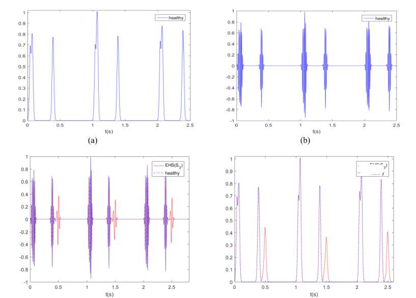
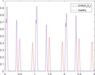
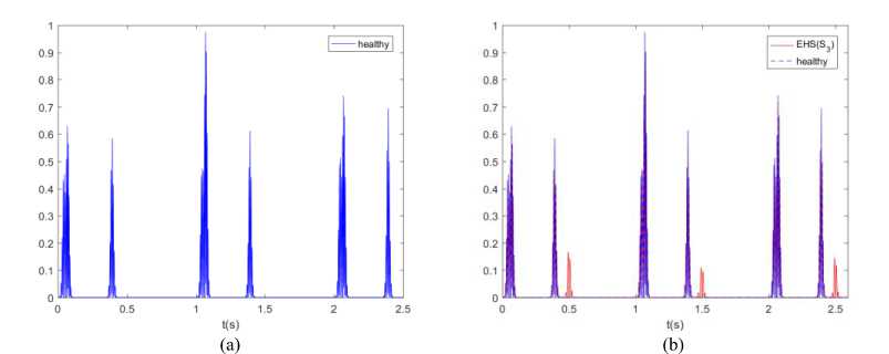
Fig.2. Examples of a PCG signals with extra heart sounds and envelope of (3), for K = 100 cardiac cycles: (a, b) healthy PCG signal, (c, d) EHS PCG signal ( s 3 ), (e, f) EHS PCG signal ( s 4 ), (g, h) EHS PCG signal ( s 3 and s 4 ).

f(s)

(h)

The objective of this study is to make use of signal processing tools to characterize PCG and EHS signals in order to correctly distinguish and identify them. The literature of signal processing offers several tools, but in our study, we will mainly be focusing on: the Root Mean Square, the envelope and the region (which is based on cyclic spectra as shown in section3.

The first tool to be tested is R oot M ean S quare ( RMS ) in the time domain which is given as:

rms

= lim          | x ( t )|² dt .

^Ц( Jo

Applying the RMS to the signals of Fig. 2 gives the following values

^(rms healthy = °.^147, rms EHS ( S 3 ) = °.1^81, rms EHS ( s 4 ) = °.^165, rms ehs ( s 3 s ₄) = °.¹⁸⁵⁾.

Of course, the signals have different RMS values even close. This last point presents the main drawback of the RMS; actually additive noise can increase the RMS and then make the comparison senseless. It should be noted that the RMS presents another limitation which concerns its dependency on the person’s subject of measure, as different persons with or without heart abnormality can have almost the same value. In order to make the RMS robust we need to follow its evolution for the same person. Consequently, this makes the RMS a relative and not a standard method. Another signal processing tool to test is the envelope. The envelopes of PCG and EHS signals are reported in Fig. 2. It is clear, from Fig. 2, that the four signals have different envelopes. Hence, we come to the conclusion that the envelope is better than the RMS, since it is an appropriate tool to differentiate between healthy PCG and each EHS. The major advantage of the envelope is the fact that it presents a unique and independent signature for a given EHS for any person. Hence, this makes the envelope a standard and independent tool.

• III.    Cyclostationary Analysis of the Proposed Pcg Models with Extra Heart Sounds

• A.  1^st-Order and 2^sd-Order Moments of t he Proposed

Model

Let’s examine the wide-sense cyclostationarity for the proposed model of (3) from the previous definitions.

We first compute the 1^st-order moment of z ( t ) and, then, the time-varying autocorrelation function. The mean

{ z ( t )} is given by:

sin Аф ^-t m z ( t ) = -T^Xl А ф _n

X ₊ M a , i ^exp l

, e [ s ± ; s ⁴ ]              '

X    q , M a,i exp l

,

( t - M - nT )² ) V ;

( t - M , - nT )²

-

I cos(2 n f (t - nT ) -ф_1)й ) +

•    mz (t) is the 1st-order moment of the Ze (t) (extra heart sounds).

= mz_h ( t ) + m_Ze ( t )

Where:

2 a,²

cos(2 n f ⁽ t ^- nT ) ^- ^ ,₀ )

•    m_zh ( t ) is the 1st-order moment of the z_h ( t )

(healthy PCG signal).

Hence z ( t ) is 1^st-order cyclostationary as m ( t ) is

T-periodic. It should be noted that m ( t ) converges to

0 when А ф moves toward n as А ф e [0, п ] .

Besides, the computation of the time-varying autocorrelation function, of the PCG signal after removing the first order cyclostationarity, is given by the following relationship:

R z ( t т ) = ^

n

X +

^{, e [ s} 1; s 2 ^]

^a a I              sin(2 A ф )                         I I   ( t - m - nT )

—j cos^fH       c^os(4 n f_t (t ^- nT ) - ф 0 ) 1 exp l-- ^{;   ;}

2 l              2 А ф I       a

₍  т 2^

^exp^{( -} ,  :) '

4a-

_     ^aa_f I               sin(2 A ф )                           I ( ( t -Mi- nT )² |    ,   т ² _

X   q^r \ ^С05⁽² п Т т ^{) +        c}os(4 n / i ⁽ t ^- nT )-2 Ф 0 ) 1 expl--^H*    ’  Iexp(^--^-)

, e [ s ₃±; s ₄± ]     ² l                   ^{2 А} Ф                            ^, (        C ,      J        4 a²

= R₄ ( t , t ) + R_Ze ( t , t )

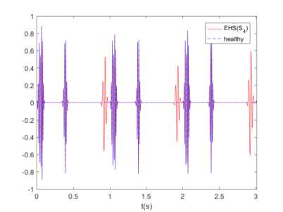
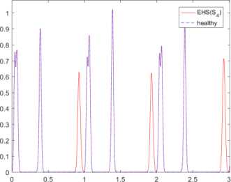
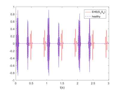
Rz (t, т)is T-periodic as well asE{x(t)} Therefore, we come to the conclusion that the signal of the proposed model of (3) is well wide-sense cyclostationary. The additive term Rz (t, т) in (4) could be used to identify extra heart abnormalities as it has a different signature of the autocorrelation function of healthy PCG signal as is shown in Fig. 3which reports numerical estimation of Rz (t, т) , for т = 0s of the synthetic signals of Fig. 2.

0.9

----EHS(S4) - - healthy

---EHS(S3S4) • - - healthy

0.5

0.2

0.2

t(s)

(c)

t(s)

(d)

Fig.3. Numerical estimate of the time-varying autocorrelation function R ( t , т ) , for т = 0 s , of the synthetic signals of Fig. 2: (a) R ( t , т ) of healthy PCG signal, (b) R ( t , т ) of PCG signal with s ₃, (c) R ( t , т ) of PCG signal with s 4 , (d) R (t , т ) of PCG signal with s ₃ and s 4 .

• B.    Cyclic Autocorrelation FunctionModel R „ ( t )

Based on the work of Gardner [3], the cyclic autocorrelation function can be defined by performing the

Fourier transform of R_z ( t,T ) with respect to t. The

Fourier transform of R _z ( t , T ) of (4) leads to:

r : ( t ) = 1

n

у ".aq wм 2T

^{, € [ s} 1 ; ^s 2 ]

T_ cos(2nfT)e "e°'1 “1 e^'2”7"'

sin(2 A " ) ^- 0 J e -

2 A"       I 2

- ",¹ n ²( a + 2 f )² e jj « ( a + 2 f i ) ft + e   "'’0

,- °»4" ^{- 2} f ⁾² e ^- j ²» ⁽ a ^{- 2 f} ) ft

8 ( a - nT - 1 ) +

'"" a

X qi 7T i €[ s ±; s ± ]          21

— T3   _2_2_,2

cos(2 n f T ) e ^{4 0} e ⁰   .

e '

- j 2 „ft ₊ sin(2 A " ) -401 I e^{2 j} "' -

2 A "

- o- ²( a + 2 f )² e j²» ( a + 2 f ) ft , + e   '"' 0

- ",¹ , ²( a - 2 f ) 2 e- j 2 n ( a - 2 f , ) ft ,

8 ( a - nT ^{- 1} )

= r ; ( t ) + r ; ( t )

With 8 (.) denotes the Dirac’s delta. The most important aspect to be observed for R „ ( t ) is the fact that it is а-discrete and nonzero only for the harmonics of T ¹ . This result confirms the second order cyclostationarity of the model of (3). It should be noted that, the term 2

V TCCT i CT a , increases when c„ increases too, this will a

2T                     i lead to an increase of second order cyclostationarity. However, sin(2A") decreases when Аф goes ton which 2A"

leads to a decrease of cyclostationarity. The additive term R; (t) in (5) corresponds to the cyclic autocorrelation function for EHS which is cyclostationary as the same as cyclic frequencies R„ (t ) cyclic autocorrelation function for healthy PCG signal. This will result in an increase of R„ (t) across the а-axis as it is shown in Fig. 4. This last point might be also used to identify extra heart abnormalities. Fig. 4 reports numerical estimation of Ra (t)of the synthetic signals of Fig. 2. As expected, it shows that the cyclic autocorrelation is nonzero only for the harmonics of T 1 i.e 1 Hz which justifies the previous theoretical results.

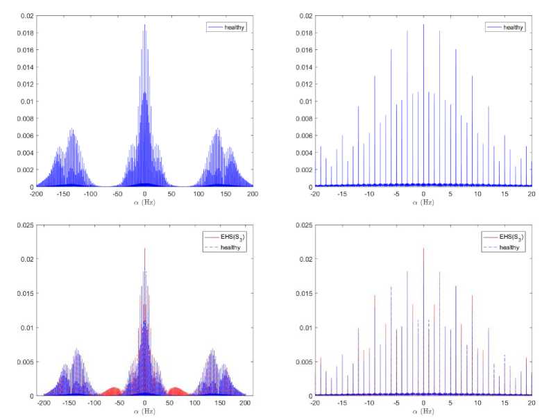
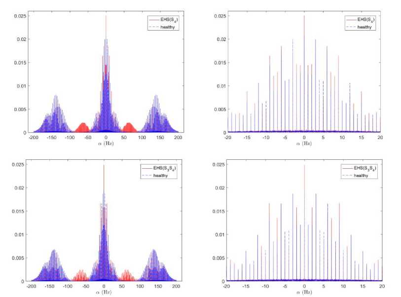
Fig.4. Numerical estimation of the cyclic autocorrelation function R ^ ( t ) of the synthetic signals of Fig. 2. The first column represents the

R ^ ( t ) and the second column represents an up-scaled of R “ ( t ) in the a -plan for т = 0 s : 1^st range- healthy PCG signal, 2^nd range- PCG signal with s 3 , 3^rdrange- PCG signal with s 4 , 4^thrange- PCG signal with s 3 and s 4 .

• C.    Cyclic spectral autocorrelation function S ^ ( f )

The cyclic spectral autocorrelation function S^ (f) sets the bases for another important second-order cyclic statistic allowing the characterization in the (f, α)-plan. As defined by Gardner [4], the cyclic spectral correlation of a cyclostationary random process in the wide sense is the Fourier transform of its cyclic correlation function with respect to t. The Fourier transform of R^ (t)of (5) leads to:

I

_ _2

nat• at

a

i <  s ±; s ± ]

2 T

s a ( f )= I

n

I

i e[ s 3 ; s 4 ]

qi

Л^ a a

2 T

-4 a ² n ²( f + fi )²   -4 a T ²( f - fi )²

e i           + e i

-a- n a eⁱ

e

- j 2яра

sin ( 2 A ^ ) -4 a²n ² f ² J 2, j^Q -a²n ²( a +2 f )² - j2лц.(a +2 f )   -2. j^ ₀ -a²n ²( a -2 f )² - j2лц.(a -2 f )

—------'- e i       <  e , e ‘         i e ' i      i + e , e ‘         i e ' i      i

2A^          [

■ ? а - nT ^{- 1} ) +

-4 a²л ²( f + fi )²    -4 a2n ²( f - fi )²

e ¹           + e ¹

2 2 2

-a^n a  - /2.пца ei e i

sin ( 2 A ^ ) -4 a ,2 n ² f ² J 2, j№   -a,²n ²( a +2 f )² - j2лц,(a +2 f ,)    -2. j№   -a,²n ²( a -2 f ,)² - j2лц,(a -2 f )

—------^L e ‘       <  e ■ e ‘         ‘ e      ‘       ‘ + e , e i         i e      i      i

■ 5 ( a - nT ^{- 1} )

2A^

= s ; ( f )+ s z ( f )

It should be noted that for the zero cyclic frequency i.e. a = 0 , the later relationship is reduced to the power spectrum density:

s 0 ( f ) = £<

n

z + ie[s±;s± ]

nCi Cai J „-4С2П2(f+fi)2    -4c2n2(f-fi)2  sin(2A^) -4c2n2(f2 + ft2) f 2JVi0 -j4nfiMi    -2JVi0 + j4nfiMi e                  I e                  I              e                    e e           I e        e

2T [                           2A^

>

£+ q 2T z e [ s ± ; s ± ]

- 4 c 2 n ²( f + fi )²     - 4 c 2 n ²( f - fi )²   sin(2 A ^ ) - 4 c 2 n ²( f ² + f ²) f ² j^ ₀ - j4f „    - 2 ^j _{V Q} + j4 „ f ^

e i            + e i           +--- ——e   i         i le i,0 e      i i + e     i,0 e      i i

2A ^              I

= sZf f ) + s 0 ( f )

As it is revealed by the formula (6), the cyclic spectral correlation S^ (f) is а-discrete and is nonzero only for a = nT-1 with resonances around ±2f . Furthermore, Sa (f) is f-continuous and presents peaks in the frequencies ±f, with i e [Sj±; s± ] О [s±; s± ], where f represents the characteristic frequencies. Fig. 5 reports numerical estimation of Sa (f) of the synthetic signals of Fig. 2 which confirms the effectiveness of the theoretical results mentioned previously.

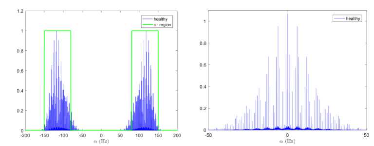
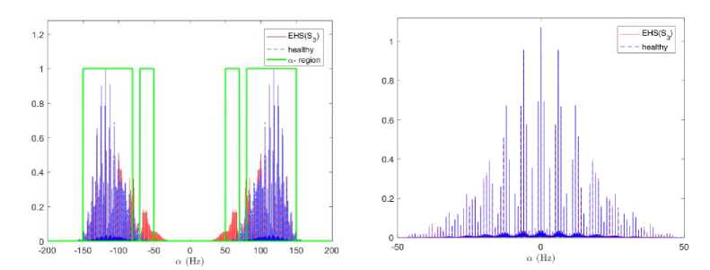
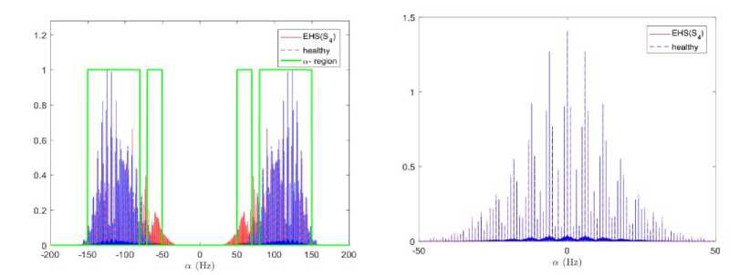
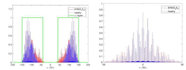
Fig.5. Numerical estimation of the spectral correlation density S ^ ( f ) of the synthetic signal, of Fig. 2. The first column represents the S ^ ( f ) for f = 0 Hz and a -region, the second column represents an up-scaled of S ^a ( f ) in the a -plan for f = 55 . 21 Hz: 1^st range- healthy signal, 2^nd range- PCG signal with s 3 , 3^rd range- PCG signal with s 4 , 4^th range- PCG signal with s 4 and s 3 .

The cyclic spectra of healthy and extra heart sounds are valuable source of information allowing the discrimination of its abnormality. One way to achieve this goal is to design a cyclic frequency region, for a given frequency, for each PCG or EHS signal. And any difference in the region width Tab. 2, even small, may help to identify the extra heart abnormality. This is possible since the heart sounds s 1 , s 2 , s 3 and s 4 have different frequencies. To design this region, we need to previously set a threshold for the cyclic frequencies where the cyclic spectrum is greater than the threshold which belongs to the region. Fig. 5 displays the cyclic spectra with characteristic region. Hence, the cyclic spectral autocorrelation function presents a very efficient characterization tool allowing the identification of different EHS.

Table 2.Band width of the cyclic frequency regions of S ^a ( f ) for healthy PCG and EHS signals.

Signals	interval (Hz)	band width (Hz)
Healthy PCG	[80 150]	70
PCG with s 3	[50 70] [80 150]	90
PCG with s 4	[40 60] [80 150]	90
PCG with s 3 and s 4	[80 150]	110

• IV.    Tests on Synthetic and Real PCG Signals with Extra Heart Sounds

• A.    Realistic Synthetic PCG Signal with Extra Heart Sounds

Normal or abnormal hearts cannot be identical in terms of parameters (3). To understand the impact of these parameters on the PCG model and to evaluate how much cyclic statistics represent a systematic signature and characteristic even for different parameters within the hearts, additional digital compilations have been done. As mentioned in section ^ , ^ _: , д ., ^ ., ^ o, A ^. and f, might vary from beat to beat for each person and from one heart to another i.e. these parameters are a demonstration of the functioning of the heart, and hence a relevant mechanism to detect either healthy or abnormal hearts. The parameters for the digital compilations are summarized in Tab. 3.

Furthermore, an additive Gaussian noise is added so that the SNR is set to the desired values. The sampling frequency for the three signals is set to 1 KHz.

Table 3. Parameters to generate three sets of realistic PCG signals according to (2).

		H ai (mv)	Oai (mv)	H l (s)	Ol (s)	P i,0 (rad)	^P i (rad)	f l (Hz)	T (s)	SNR (dB)	К
-a	S i	0.45	0.20	0.0446	0. 0143	2.83	П 6	67.86	0.78	25	100
	— si	0.93	0.10	0.0748	0.0111	3.14	П 6	76.59
	S 2+	0.70	0.09	0.3676	0.0111	3.14	П 6	69.12
	— S 2	0.51	0.09	0.3915	0.0111	0.00	П 6	62.83
	S 3+	0.48	0.05	0.4791	0.0095	0.14	П 6	36.92
	— S3	0.42	0.02	0.5013	0.0127	2.08	П 6	43.27

-a	s1+	0.33	0.09	0.0366	0.0127	2.00	π 4	63.21	0.73	20	100
	s 1-	0.80	0.08	0.0700	0.0111	3.14	π 4	68.05
	s 2 +	0.53	0.02	0.3804	0.0127	0.18	π 4	62.27
	— s2-	0.52	0.07	0.3756	0.0127	3.14	π 4	66.98
	s 4+	0.32	0.05	0.6907	0.0111	1.09	π 4	27.10
	s 4 -	0.31	0.06	0.6971	0.0127	1.00	π 4	29.19
-a	s1+	0.43	0.04	0.25	0.0175	2.23	π 3	65.97	0.79	15	100
	s 1 -	0.76	0.15	0.50	0.0127	3.14	π 3	71.94
	s 2 +	0.43	0.03	2.36	0.0064	3.14	π 3	67.36
	— s 2-	0.33	0.08	2.45	0.0271	3.14	π 3	66.98
	s 3 +	0.40	0.05	0.5077	0.0207	1.11	π 3	38.92
	s3-	0.26	0.02	0.5093	0.0143	1.20	π 3	46.92
	s 4 +	0.19	0.02	0.7448	0.0239	1.09	π 3	27.10
	s 4-	0.18	0.01	0.7512	0.0143	1.00	π 3	28.19

2nd data set                                       3rd data set                                       4th data set

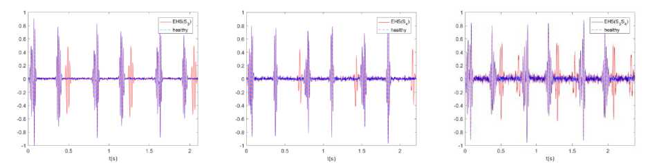
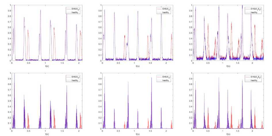
Fig.6. 1st range- realistic PCG signals, 2nd range- envelope of PCG signal and 3rd range- time-varying autocorrelation functions.

2nd data set

3rd data set

4th data set

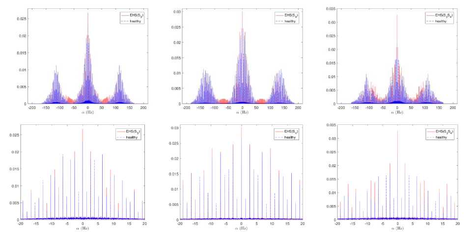
Fig.7. A numerical estimate of the cyclic autocorrelation functions R ^α ( τ ) : 1^st range- R ^α ( τ ) in the α -plan for τ = 0 s and 2^nd range- up-scaled of

R ^α ( τ ) in axis α for τ = 0 s , of each synthetic PCG signal.

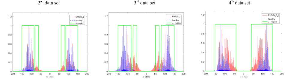
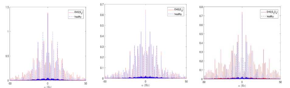
Fig.8. A numerical estimate of the spectral correlation density S ^α ( f ) : 1^st range- S ^α ( f ) in the α -plan, for f = 0 Hz and 2^nd range- up-scaled in axis α for f = 66 . 56 Hz; f = 59 . 57 Hz; f = 43 . 94 Hz), of each synthetic PCG signal.

Second order statistics reported in Fig. (6, 7 and 8), confirm the cyclic behavior of the three PCG signals even if the cyclic periods are different. It should be noted that the cyclic statistics are not sensitive to noise since the noise is supposed to be stationary. The results of the envelope and the second order statistics applied to 2nd, 3rd and 4th data sets are similar to the ones of 1st data set, we come to the conclusion that the envelope and the second order statistics give an effective framework for detecting and identifying EHS.

• B.    Real PCG Signals with Extra Heart Sounds

The second order statistics for real PCG signals (healthy and EHS) will indicate the matching of the proposed model of (3). To do this, we make use of data sets provided from [21] which have been gathered from a clinic trial in hospitals using the digital stethoscope DigiScope.

The second order statistics reported in Fig. (9, 10 and 11) show that the three real PCG signals (healthy and EHS) are well wide-sense cyclostationary. Furthermore, the 2nd and 3rd real data sets corresponds respectively to the EHS s3 and s4; and have similar time representation, envelope, cyclic frequency region and second order statistics to the corresponding synthetic signals of (3) shown respectively in Fig. (2-c) and Fig. (2-e). In addition, the time representation and the envelope of each heart beat has Gauss-like shapes which approve the validness of the proposed model of (3). These results prove the matching of the proposed model of (3) with reality.

2nd data set

3rd data set

4th data set

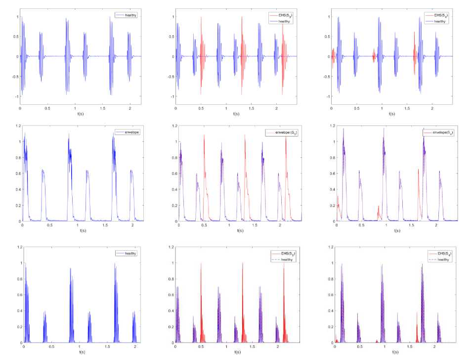
Fig.9.1st range- realistic PCG signals, 2nd range- envelope of PCG signal and 3rd range- time-varying autocorrelation functions.

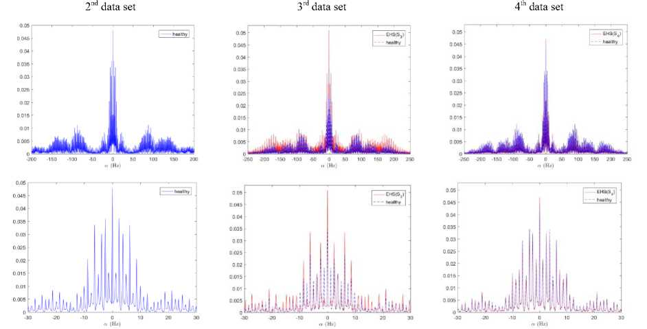
Fig.10. A numerical estimate of the cyclic autocorrelation functions R ^α ( τ ) : 1^st range- R ^α ( τ ) in the α -plan for τ = 0 s and 2^nd range- up-scaled of

R ^α ( τ ) in axis α for τ = 0 s , of each synthetic PCG signal.

2nd data set                                     3rd data set                                       4th data set

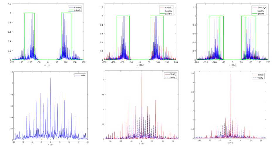
Fig.11. A numerical estimate of the cyclic autocorrelation functions Rα (τ): 1st range- Rα (τ) in the α-plan for τ = 0 s and 2nd range- up-scaled of Rα (τ) in axis α for τ = 0 s, of each synthetic PCG signal.

• V.    Conclusion

In this study, we have developed an explicit analytical model to better describe PCG signals with extra heart sounds over several cardiac cycles. Actually any trouble in the heart functioning, namely extra heart sounds, will directly influence second order cyclic statistics since cyclic statistics are not sensitive to stationary additive noise and, thus, allow the detection and the identification of extra heart sounds. The findings of this study suggest that the tested signal processing tools, evaluated over the developed analytical model, are reliable to be used as alarms to alert cardiologists to the presence of extra heart sounds or even to suspect early heart abnormalities.