Cyclic Analysis of Phonocardiogram Signals

The Phonocardiogram signal (PCG) is a temporal representation of the acoustic sound of the heart vibration. It is a considerable source of information that can lead by its analysis, to the detection and the identification of several heart abnormalities. A PCG signal in the healthy case consists of two fundamental sounds, i.e. the first heart sound s 1 and the second heart sound s 2 . These two fundamental sounds are derived from the mechanical functioning of the heart and are due to the closing of the valves and the turbulent passage of blood [14]. There are other sounds than s 1 and s 2 that may correspond to diseases or problems in the heart valves. Although some diseases tend to be recognized with difficulty, by using a stethoscope, they are all reflected on the patient PCG signal. That is why we resort to this type of signals to identify the state of the heart.

Regarding the analysis of digital PCG signals, all related works in this area are based on time-frequency analysis [12, 9]. To the best of our knowledge, the existing models do not exploit the periodic character of the heart functioning. As a matter of fact, the heart sound is a series of repeated mechanical actions. The repetition is not exactly periodic but is considered quasi-periodic. It means that the vibration wave recordings are cyclostationary [1, 13, 16]. Many natural or man-made processes in various fields arise from periodic phenomena, as mechanics, telecommunications, radio astronomy, econometric, … These processes, although not periodic functions of time, give rise to random data whose statistics vary periodically with time and are called cyclostationary processes [20].

A stochastic signal x ( t ) of mean E{ x ( t )} and timevarying autocorrelation function

Rx (t ,T) = E {x (t - T / 2) x * (t + т / 2)}, where the superscript * denotes complex conjugation, is said to be wide-sense cyclostationary with T0-period if both E{x(t)} and R (t,t) are periodic over time t with To-period [3], i.e. E{x(t)} = E {x(t + To)} for all t

Rx (t,t) = Rx (t + To ,t) for all t, t.

The time-varying autocorrelation function is, thus, periodic over tand can be expanded in Fourier series:

+^            j 2n—t

R x ( t , T ) = 2 R x / T 0 ( T ) e    ^T0

n =—^

where R x / ^{T o} ( t ) is known as the cyclic autocorrelation function and is given by:

n

1 r T _o/2             ^- j ²ⁿ~ t

R"/To(t) = -   0  Rx (t,t)e    T0 dt

• ^x                - T /2 ^x

T0   0

where n / T , n e 0 are the cyclic frequencies.

The Fourier transform of the cyclic autocorrelation function with respect to the cyclic frequency α gives rise to the spectral correlation density function:

s ? ( f ) = Г* « ? ( г ) e - j² '"' d r . -to

In this context, several models representing the functioning of the heart sounds were presented in the literature [14, 18, 8]. However, these models are limited to a single cardiac cycle, and hence remain uncompleted. Thus, the purpose of this study is to introduce a coherent cyclostationary and Gabor kernel based model for a whole description of PCG signals. The proposed model takes into account the fluctuation of the heart beats from one cycle to another. The motivation behind is to define a framework, utilizing cyclic statistic due to noise robustness, for a full description of PCG signals, which leads to an easy and efficient early identification of certain heart abnormalities. The validation of the proposed model and its capacity to reflect the heart functioning is tested over synthetic and real data sets.

This paper is organized as follows. Section 2, describes the modeling of PCG signals. Section 3 concerns the analytical study of the proposed model, some simulation results are also presented in this section in order to confirm the theoretical analysis. Section 4 focuses on the validation of the computed cyclic statistics on synthetic and experimental PCG signals. Finally, Section 5 is dedicated to conclusions.

• II.    PCG M odeling

• A.    Context

A PCG beat mainly consists of two distinct sounds, s 1 and s 2 , sample waveforms of which are depicted in Fig. 1. The need of an adequate framework, for the detection and the classification of abnormalities in the heart functioning, has pushed researchers to be interested in the modeling of the PCG signals. Therefore, modeling the shape of the heart sounds has been studied by many authors: the chirp model [10, 11, 17], the damped sinusoidal model [5, 2], and the modified Prony model [6]. To our knowledge, all related models are limited to a single cardiac cycle and give no information about the behavior of heart sounds for the remaining cycles. The motivation of this work is to build up a mathematical model able to produce the shape and the quasi-periodic character of heart sounds.

• B.    Established PCG Model

2.0, ²    I ^{x 1}       '

Among the existing PCG models, the ones based on Gabor and Laplace kernels [18, 19, 7, 8, 10] seem to be more realistic. The Gabor kernel, which is actually a Gaussian-damped sinusoidal wave, offers the possibility, through        five        adjustable        parameters

( a_t , О , ^ , f and ^ ) , to exactly reproduce the shape of any heart beat.

The model of (1) makes use of two Gabor kernels to represent each heart sound s 1 and s 2 . Therefore, one heart beat of PCG signal can be modeled with four kernels as given bellow (Fig. 1):

Z a exP i e[ $1 ; $2 ]

(t--^ )- |cos ( 2n ft - ^ )       ⁽¹⁾

Where

• f and фг are respectively the frequency and the phase shift of the sinusoid terms.

•  a,, Д-, and О are successively the amplitude, the center and the width which represent the parameters of the Gaussian terms.

± is a superscript indicating the two Gabor kernels which are used for modeling each heart sound, with

[ $ ± ; $ ± ] = [ $ 1 , $ + ; $ 2 , $ 2 ⁺ ] .

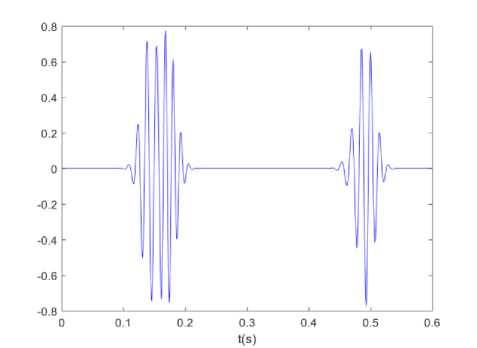
Fig.1. Example of healthy PCG signal for a single heart cycle of (1).

• C.    Modified PCG Model

The model of (1) represents the PCG signal for a single cardiac cycle. Unfortunately, this representation is not enough to make a full characterization of the heart in a limited time. Hence, the idea of the proposed model, to achieve a whole description is to jointly combine Gabor kernels, for modeling the shape of heart sounds, with some randomness to reproduce the fluctuations occurring in the heart functioning for every cardiac cycle. This combination leads to the model given by the following expression:

z ⁽ t ) = Z   a in exp

±  ± ie[$| ,$2],n

⁽ t ^{Ц 1} 2 nT ) ] ^cos ( 2 n f i ⁽ t ^- nT ) ^- V in )

Where

• •    The index n stands for the cardiac cycle.

• •    T is the cardiac cycle duration.

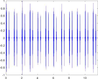
The random behavior in z(t) comes simultaneously from the parameters at n and V „ . This means that the amplitude and the phase for each heart sound might change for any cardiac cycle. Where a is the amplitude of Gabor kernel, for the ith heart sound and the nth cardiac cycle, which follows a Gaussian law N (Hat, ^ whereas the phase ф/  follows a uniform law inside the interval [ф 0 — Аф, ф 0 + Аф] with is Афе [0, п] and фу the ith initial phase. An example of the proposed model of (2) is given by Fig. 2 where the parameters are showed in Tab. 1.

Moreover T = 1 s , K = 100 cardiac cycles and the sampling frequency f is set to. 1000 Hz .

Table. 1. Mean values of the phonocardiogram (PCG) model parameters according to (2).

		Ц ат. (mv)	^ ai (mv)	№ (s)	O i (s)	V i,o (rad)	ktp i (rad)	f i (Hz)
-a	S1+	0.8	0.02	0.0414	0.0127	2.77	П 10	66.66
	— S1	0.8	0.15	0.0716	0.0127	1.73	П 10	78.85
	$2+	0.8	0.10	0.3836	0.0143	3.14	П 10	66.92
	— $2	0.9	0.07	0.3883	0.0143	3.14	П 10	71.19

t(s)

Fig.2. Example of a healthy PCG signal of (2), which shows the almost periodic behavior of PCG signals.

• III.    C yclostationary A nalysis of the P roposed PCG M odel

• A.    1^st-Order and 2^nd-Order Moments

Let us check the wide-sense cyclostationarity for the proposed model using the previous definitions. We first start compute the 1^st-order moment of z ( t ) and, then, the time-varying autocorrelation function. The expectation E{ z ( t )} is given by:

sin Аф                  .  ( t  Ц-  nT )

m(t) =         S   ^a,i exP(—     ;       )cos(2nf1 (t - nT) - ф,о)              (3)

^А Ф i e [ s ± , s ± ], n                      2 ^1

m ( t ) is T-periodic which indicates that z( t ) is 1^st-order cyclostationary. It should be noted that m ( t ) converges to 0 when А ф moves toward n as. А ф e [0, п ] .

Besides, the computation of the time-varying autocorrelation function, of the PCG signal after removing the first order cyclostationarity, is given by the following relationship:

R- ⁽” ¹ = S ^ {

sin(2 A ф )

cos(2 n f j ) +-------- cos ( 4 п f ( t — nT ) — 2 ф _g)

( ( t — ^ — nT )²

expl--------

V       ^i

2Аф

( т 2 ) exp —

V  4^2 J

}

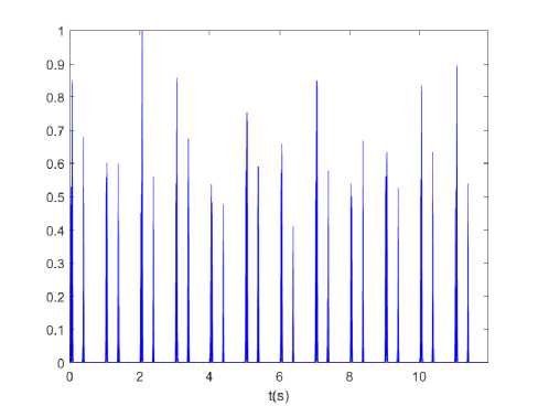
Fig.3. A numerical estimate of the time-varying autocorrelation function

R ( t , T ) for T = 0 S , of the synthetic signal of Fig. 2.

R_z ( t, T ) is T-periodic as well as E{ z ( t )} . Hence, we come to the conclusion that the signal of the proposed model of (2) is well wide-sense cyclostationary. Moreover, Fig. 3 reports a numerical estimator of R_z ( t , T ) , of the synthetic signal of Fig. 2 which confirms the previous theoretical result.

• B.    Cyclic Autocorrelation Function R ^ ( t )

According to Gardner [3], the cyclic autocorrelation function can be defined by performing the Fourier transform of R_z ( t, T ) with respect to t. Thus, the Fourier transform of R_z ( t, T ) of (3) leads to:

—

t

2  222

4c  -с п а  — j 2пац.

e 1 e 1 e 1 +

R ( t ) = ^ "^ <  z ^ 2^T

f_ sin(2Аф) 4c2 2Аф

( ² Ф 0    7 7      7

e ' ^— с ² п ²( a —2 f_t )² j2п(а —2 f_t ) ц

V

^{2 j}^i 0     7 7        7

e ,     с ² п ²( a +2 f .)²  — j 2п (a +2 f ) ц

+--e 1          1 e

> 5 (a — nT ^{— 1})?

/

With 5 (.) denotes the Dirac’s delta.

The first thing to note is that R ^ ( t ) is а-discrete and is nonzero only for the harmonics of T ¹ . This point confirms the second order cyclostationarity of the model of (2). Also, the term " ^ " i  increases when c _t

22T increases too, this will result in an increase of cyclostationarity. However, sin(2Aф) decreases when 2Аф

Аф goes to n which leads to a decrease of cyclostationarity.

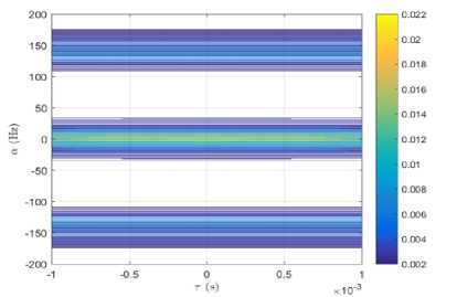
Fig. 4 reports a numerical estimator of R ^ ( t ) of the synthetic signal of Fig. 2. As expected from theory, the figure shows that the cyclic autocorrelation is nonzero only for the harmonics of T ¹ ie 1 Hz which validates the previous theoretical results.

-200    -150   -100    *50      0 .    50     100    150    200

(a)

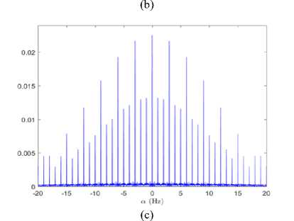
Fig.4. A numerical estimate of the cyclic autocorrelation function R- O. ( T ) of the synthetic signal of Fig. 2: (a) R ^ ( T ) as a function of а and t, (b) R a ( T ) in а-plan for T = 0 5 , (c) zoom of R ^ ( T ) in the а-plan for T = 0 5 .

• C.    Cyclic Spectral Autocorrelation Function S ^ ( f )

Sa (f) represents another important second order cyclic statistic allowing the characterization in the (f, a) -plan. As defined by Gardner [4], the cyclic spectral correlation of a cyclostationary random process in the broad sense is the Fourier transform of its cyclic correlation function with respect to t. So, the Fourier transform Ra (t) of (4) leads to:

Sa (f)=1 ""

i,n   4T

( e ■": ^{2( f} - fi ⁾² ₊ e -Цк ^{2( f} + fi ⁾² ) e ~"²n ² a ² e - j 2 кащ +

sⁱⁿ⁽2A ^ )   - "П ² f ² / 2M,0   ."П ² ( a - 2 f -)² - j2 n ( a - 2 f ) д

e    ee     e

2A^           \

+ e ^{- 2} ^ e ^- "* ^{n 2( a + 2 f )}2 e ^- j^{2 n ( a + 2} f ) Д

j > 8 (a - nT-1)

It should be noted that for the zero cyclic frequency i.e. a = 0 , the later relationship is reduced to the power spectrum density:

sZ( f)=1 ""

i,n   4T

< e"^ ^{2 (} f ^- fi ^{) 2} + e

,4 " 2 n ² ( f + fi ) ^{2    sin(2 A} ^ )   - 4 " ² n ² ( f ² + f_t ²)   ² j i ,o j4 n f i ^ i

•                +    _ e                  e e         I e

2 A ^

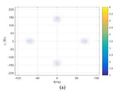
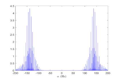
As it is shown by the relationship (5), the cyclic spectral correlation S _z ^a ( f ) is a-discrete and is nonzero only for a = nT ^{- 1} with resonances around ± 2 f . Furthermore, S _z ^a ( f ) is f-continuous and presents peaks in frequencies ± f , with i G [ s ± , s ± ] , where f represents a characteristic frequency.

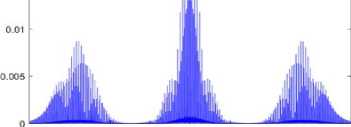
Moreover, Fig. 5 reports a numerical estimator of S _z ^a ( f ) of the synthetic signal of Fig. 2 which confirms the effectiveness of the theoretical results mentioned previously.

(b)

,^-2 j ^ -,0 _e ^{- j4 n f}i M i ) ,

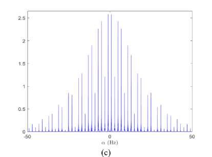
Fig.5. A numerical estimate of the spectral correlation density S a ( f ) : (a) S a ( f ) a function of ( a , f) , (b) S _z ^a ( f ) in the a -plan for f = 0 Hz , (c) zoom of S a ( f ) in axis a for f = 73 . 24 Hz , of the synthetic signal of Fig.

• IV.    E valuation on S ynthetic and E xperimental P cg S ignals

• A.    Realistic Synthetic PCG Signals

Additional simulations have been made in order to confirm the cyclostationary behavior of the mathematical model of (2) regarding its parameters. Actually, the parameters

Mai, "ai, Mi , "i, ^i,0 , A^i and f mentioned in subsection II.C, might vary from beat to beat and for each person i.e. these parameters represent the functioning of a unique heart.

Two healthy hearts cannot have exactly the same parameters. Other data sets are necessary to understand the influence of these parameters on the PCG model and to evaluate how much cyclic statistics represent a coherent signature and characteristic even for different hearts (different parameters), and thereby a suitable to recognize healthy hearts. The parameters for the simulations are listed in Tab. 2. Moreover, an additive Gaussian noise is added such that the SNR is set to the desired values. The sampling frequency for the three signals is set to 1000Hz.

Table. 2. Parameters to generate three sets of realistic PCG signals according to (2).

		H al (mv)	O al (mv)	H l (s)	Ol (s)	Pl,0 (rad)	^P l (rad)	f l (Hz)	T (s)	SNR (dB)	К
-a	Si	0.45	0.25	0.0446	0.0223	2.83	П 6	67.86	0.83	30	100
	— si	0.93	0.17	0.0748	0.0111	3.14	П 6	76.59
	S2+	0.70	0.20	0.3676	0.0111	3.14	П 6	69.12
	— S2	0.51	0.09	0.3915	0.0111	0.00	П 6	62.83
-a	S1	0.33	0.03	0.23	0.0127	0.0127	П 4	63.21	0.76	20	100
	— si	0.80	0.19	0.44	0.0111	0.0111	П 4	68.05
	S2+	0.53	0.02	2.39	0.0127	0.0127	n 4	62.27
	— S2	0.52	0.05	2.36	0.0095	0.0095	n 4	66.98
-a	s1	0.43	0.04	0.25	0.0175	2.23	n 3	65.97	0.65	10	100
	— si	0.76	0.15	0.50	0.0127	3.14	n 3	71.94
	S2+	0.43	0.03	2.36	0.0064	3.14	n 3	67.36
	— S2	0.33	0.08	2.45	0.0271	3.14	n 3	66.98

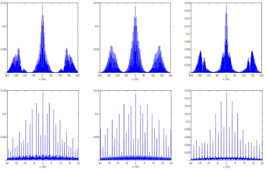
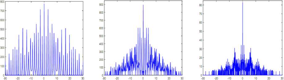
Fig.7. A numerical estimate of the cyclic autocorrelation functions R ^α ( τ ) : 1^st range- R ^α ( τ ) as a function of α and τ, 2^nd range- R ^α ( τ ) in the α-plan for T = 0 S , and 3 rd range- zoom of R a ( t ) in axis a for T = 0 S ;of each synthetic PCG signal.

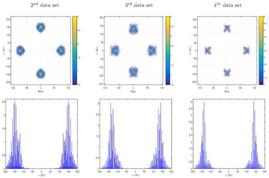
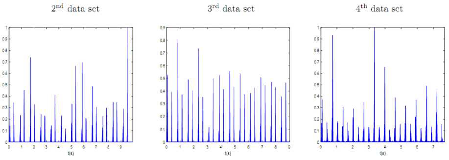
Fig.6. A numerical estimate of the time-varying autocorrelation functions of each synthetic PCG signal.

2nd data set

3rd data set

4th data set

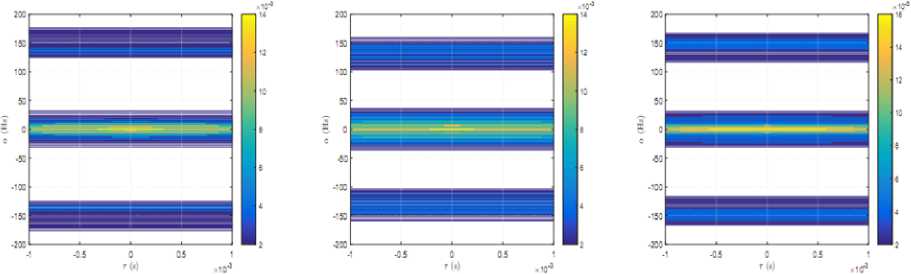
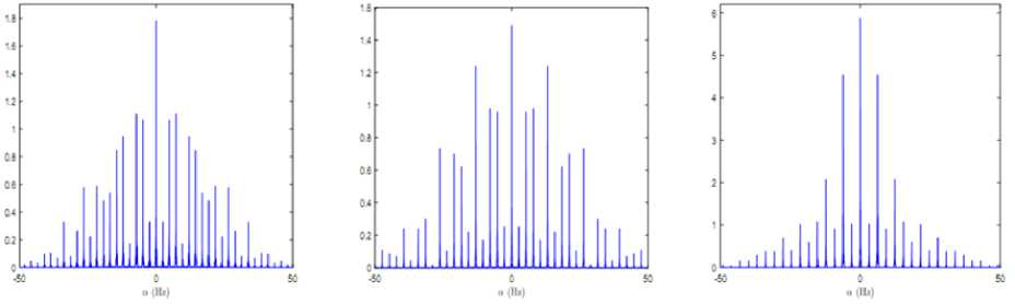
Fig.8. A numerical estimate of the spectral correlation density S ^ ( f ) : 1^st range- S ^ ( f ) as a function of a and f, 2^nd range- S ^ ( f ) in the а-plan, for f = 0 Hz and 3^rd range- zoom in axis a for ( f = 76.66 Hz , f = 67.87 Hz , f = 71.77 Hz ) ; of each synthetic PCG signal .

The second order statistics reported in Figs. (6, 7 and 8), confirm the cyclic behavior of the three PCG signals even if the cyclic periods are different. It should be noted that the cyclic statistics are not sensitive to noise since the noise is supposed to be stationary.

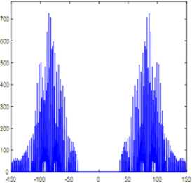
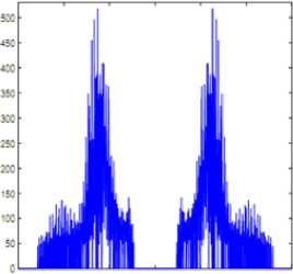
• B.    Experimental PCG Signals

The estimations of second order statistics for real PCG signals will indicate the matching of the proposed model of (2) with reality. To do this we make use of data sets provided from [15] which have been gathered from a clinic trial in hospitals using the digital stethoscope DigiScope.

The second order statistics reported in Figs. (9, 10 and 11) show that the three real PCG signals are well wide-sense cyclostationary . This result matches with the one of synthetic PCG signals which proves the effectiveness of the proposed model of (2). It should be noted that the last two real PCG signals are very noisy. The perturbations in cyclic autocorrelation function and the spectral correlation density of the last two real PCG signals may be explained by the strong fluctuation of the cyclic period i.e. cardiac cycle. Furthermore, the spectral correlation density functions are thresholded in order to exclude noise due to the estimator since signals have a small number of samples.

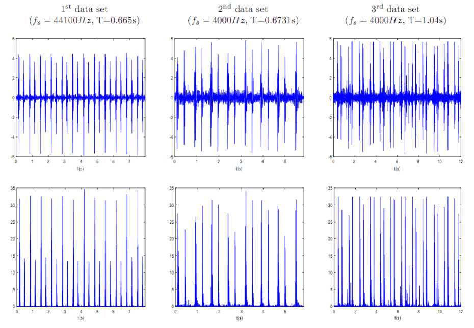
Fig.9. 1st range- time representation of the real PCG signals and 2nd range- time-varying autocorrelation function for each real PCG signal.

Fig.10. The cyclic autocorrelation functions: Rα(τ) of the three real PCG signals: 1st range-Rα(τ): as a function of α and τ, 2nd range- Rα(τ) in the α-plan for τ = 0s and 3rd range- zoom of Rα(τ) in axis α for τ = 0s .

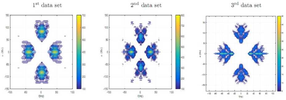
jsc .ео 40 о so юс iso

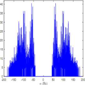
O (Hl)                                                                 О (Hl)                                                                 о (Hl)

Fig.11. The spectral correlation density S ^ ( f ) of the three real PCG signals: 1^st range- S ^ ( f ) as a function of a and f, 2^nd range- S ^ ( f ) in the a-plan for f = 0 Hz and 3 rd range- zoom in axis a for ( f = 43 Hz , f = 26.91 Hz , f = 29.29 Hz )

• V.    C onclusion

In this study, we introduced a new PCG model allowing a better description of heart beats over several cardiac cycles. The effectiveness of the model was validated over synthetic and real PCG signals. We proved the wide-sense cyclostationarity of the model that allows an accurate characterization of PCG signals as cyclic statistics are not influenced by stationary additive noise. Hence, any trouble in the heart functioning, even small, will influence second-order cyclic statistics. This modification could be used as an alarm that alerts cardiologists to suspect early heart abnormalities.