Cyclic Sparse Greedy Deconvolution

Published Online November 2012 in MECS

In this study we focus on Cyclostationary (CS) signals made of periodic random impulses. Given the Impulse Response (IR), the aim is to retrieve the original object which has been distored by passage through a known linear and time-invariant system in presence of noise. Indeed, improving the resolution of the signal and the Signal to Noise Ratio (SNR) from the knowledge of the IR corresponds to a deconvolution problem. The deconvolution of cyclostationary signals has been addressed by severals authors with different approaches. In [1], a bayesian deconvolution algorithm based on Markov chain Monte Carlo is presented. Cyclic statistics are often used for deconvolution, in [2], [3] the deconvolution is based on cyclic cepstrum, whereas, in [4], [5] the deconvolution is based on cyclic correlation. Actually, signal deconvolution is known to be an ill-posed problem as the IR acts as a low-pass filter and the convolved signal is noisy. Fortunately, regularization techniques allow to retrieve satisfactory solutions accounting for a priori information on the original object. Analysing periodic random impluse signals in details uncover another a priori information which is sparsity, this is because only few impulses are nonzero. Note that sparsity is interesting as well as cyclostationarity.

Our work consists on extending sparse approximation to CS signals with periodic random impulses, where the aim is to find jointly a sparse approximation of each cycle, accounting for the same elementary signals in each approximation, but shifted with a multiple of the cyclic period and with different coefficients. However, we insist in the application of cyclosparse approximation to deconvolution.

The paper is organized as follows, section II defines problem statement. In section III, we summarize the statement of sparse and cyclosparse approximation problems. The main contribution of this paper is described in sections IV and V, where we, respectively, introduce the concept of cyclosparsity and address the problem of deconvolution of cyclosparse objects. Also, in section IV, we point-out the link with cyclosparse deconvolution. Such a cyclosparse model is taken into account in the sparse deconvolution by greedy algorithms in section V, which fortunately reduces significantly the computation cost. In this paper, we focus on greedy algorithms and we propose to test some of these algorithms, namely Matching Pursuit (MP) [6] and Orthogonal Matching Pursuit (OMP) [7] on the same statistical basis, i.e. with the same stopping rule deduced from statistical properties of the noise. These algorithms are summarized in the cyclosparse case as well. Also it seems to be necessary to obtain satisfactory deconvolution results, as shown in the simulation results section VI.

• II.    Problem statement

Consider the situation where a known system h( t) is excited by a CS signal x (t) consisting of periodic random impulses. By periodic, we mean that the signal can be partitioned into portions of length T (which is known as the cyclic period of the signal) with d impulses in each portion. Moreover, the delay factor i of the ith impulse x , is constant for all portions. Note that in general т , will be different for different i although in most of the cases they may be integral multiples of a constant t. An example of x( t) is shown in Fig. 1 with d = 5. Note that the impulse with т₃ as delay factor is nonzero for the first and second cycles (x_t , ₃,x₂ , ₃ * 0) whereas for the third cycle it is of null amplitude x₃ , ₃ = 0.

The output of the system described above can be written as,

У (t) = Sf o ¹ St 1 x_tik h( t - (т_к + iT)) + n(t) (1)

Where d is the number of effective impulses in the period with _, and т being their amplitude and delay factors respectively. К denotes the number of period per signal and the sub-index i stands for the period index, so

_, represents the impulse with τ as delay factor in the ith -period. ( ) represents the random noise of the system.

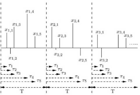
Fig. 1. Example of cyclosparse signal.

• III.    FROM SPARSE TO CYCLOSPARSE APPROXIMATION

• A.    Sparse approximation

The problem of sparse signal approximation consists in approximating a signal as a linear combination of a limited number of elementary signals (atoms) chosen in a redundant collection (dictionary). It can be written as: Find sparse such that Φ ≈  , where corresponds to measured data and Φ is a known matrix with atoms {  }   … as columns. Sparse approximations have to deal with a compromise between a good approximation and the number of involved elementary signals. Such compromise results mathematically to minimize the criterion:

( )=‖ -Φ ‖ + ‖ ‖                     (2)

Where ‖ ‖ = Card{ ,   ≠ 0}, is the number of nonzero components of . The parameter controls the trade-off between the sparsity of the solution and the quality of the approximation. The lower is , less sparse is the solution and better is the approximation.

Minimizing such a criterion is a combinatory optimization problem which is NP hard. Two approaches are generally used to avoid exploring every combination: Greedy algorithms and convex relaxation algorithms.

• B.    Cyclosparse approximation

The extension of sparse approximation for CS and sparse signals will be studied in this article. A cyclosparse solution is given by minimizing the following criterion:

( )=∑  ‖ -Φ     ‖ +   ‖ ‖ ,           (3)

with =0,…,  -1.

and     denote respectively the number of cycles/periods and the cyclic period.

The inner norm encourages diversity along the cycles of so the , mixed-norm measures the cyclosparsity along the whole signal as illustrated in Fig. 1. The choice of , mixed-norm result will be illustrated in the next section.

• IV.    CONCEPT OF CYCLOSPARSITY

• A.    Definition

A process x is said to be cyclosparse if

‖  ‖  ≤   ‖  ‖  ,                                               (4)

With can be reshaped as × matrix.

• B.    Proof

Let us first introduce the following notations:

A Xt, = x((i —1)T+1:i T)  with 1

a  x: ^ = x( к,к + T ,k + 2T,... ,k + (K — 1)T)

with 1≤  ≤ sweeps all kth elements of each period(a total of elements).

The -norm of is defined as follows

• ‖  ‖  =∑   |   |(5)

As is standard, |   |  =1 if ≠0 and |   |=0

=0 .

Using these notations, the equation 5 can be written as, ‖ ‖  = ‖  ,:‖  +‖  ,:‖  +⋯+‖

=∑| , | + ∑| , | +⋯+∑| k=l         k=lk=l

=|  , |+|  , | +⋯+|

+|  , | +|  , | +⋯+|

+ ⋮    +  ⋮  +⋯+⋮

+|  , | +|  , | +⋯+|

Also, we can write

• ‖ ‖  ≤ (|max |  , || + |max |  , ||+⋯+

|max |

T

≤ ∑|max| , || = ‖max| ,:|‖  =‖ ‖ k=l max |  ,:| stands for -norm of along dimension of for each value of the period indexed by . The composite norm ‖max | ,:|‖ is the mixing norm  , of which the minimization encourages first diversity along and then sparsity of the resulting vector.

• V. DECONVOLUTION IN CYCLOSPARSITY CONTEXT

• A.    Problem formulation

Let us first specify the boundary condition accounted for in the convolution operator. We assume that the object is zero-valued outside the signal to reconstruct of size . The convolution of the object leads to a signal of size =    +    -1. Thus, the dictionary is given by the (   +   -1)× Toeplitz matrix H where the columns are built from the IR ℋ.

Therefore, Eq. 1 can be written with matrix notations as,

= H D +

= H̃+

H H =  (HT ) with D is the cyclosparsity operator

D ^T =D =∑

‖‖

∑

/ , ^п+тТ^^п+тТ _m=0 п=1

= diag (∑    ∑‖ ‖ , where are the canonical basis vectors and is the index of the nth impulse with as factor delay. Thus, H̃ is a matrix with particular structure i.e. the nonzero columns for each cycle are deduced by shifting the columns of the first cycle with a multiple of the cyclic period . Hence, H̃ points out the cyclosparsity property in the convolution case.

It should be noted that both approaches used to avoid exploring every combination of the sparse approximation problem can be extended to cyclosparse context: greedy algorithms and convex relaxation. In this paper, we focus on greedy algorithms.

• B.    Cyclosparse greedy algorithms

Let the sub-matrix H _Ʌ built-up from the columns of H where the indices are in Ʌ, =H , and Ʌ^{( )} is the set of the selected indices at iteration . The vectors are defined as follows, =[ ,…, ], y =[ ,…, ],

=[ ,…, ] and =[ ,…, ] which denotes the residual. , and stand respectively for the length of , and ℋ . Finally, let the vector = [0,1,…․,( -1)] be the vector of period indices.

Greedy algorithms are iterative algorithms composed of two major steps at each iteration: 1) the selection of an additional elementary signal in the dictionary; 2) the update of the solution and the corresponding approximation. A stopping rule helps to decide whether to stop or continue the iteration.

Let ( ) be the solution of the kth iteration, ( ) being its coefficients at indices Ʌ and ( ) = - H ( ) the residual corresponding to this solution (approximation error). The typical structure of a greedy algorithm is: Initialize =0, Λ( ) =∅ and ( ) =  .

Iterate on =  +1 until the stopping rule is satisfied:

^ Select the index i ( ^k) corresponding to an atom improving the approximation.

^ Update the solution x^ , with non-zero elements at indices Λ( ) =Λ(   ) ∪{ ( )}, and the corresponding residual ( ).

The various algorithms differ on the selection or the updating steps.

Cyclo-Matching Pursuit (Cyclo-MP) is the extension of the MP [6]. The additional atoms (at most atoms) jointly maximize the scalar product with the residual. The update corresponds to an orthogonal projection of the residual on the selected atoms, so only the solution at the selected indices is updated. Note that with such a scheme it is possible to select already selected atoms. In order to avoid overloading equations, the index ^{( )} will be replaced by ^{( )} in the following.

^ Selection of К atoms: Л^(к) = Л^(к “ ¹ ) U{i^},

( ) =arg max ∑    |        (   )|

^A Update:

solution:

(( )) =   (( ) )+(   ( )   ( ))       ( )   (    )

LmT lmT ' mT mT / LmT residual:

( ) =    (     )-    ( ) (   ( )    ( ))       ( )   (     )(8)

^LmT X ^гтТ ^LmT / ^гтТ

• -^  Stopping criterion

Cyclo-Orthogonal Matching Pursuit (Cyclo-OMP) is the extension of the OMP [7]. The Cyclo-OMP differs from the Cyclo-MP on the updating step as an orthogonal projection of the data on the whole selected atoms is performed. This avoids the selection of already selected atoms but increases the computation cost as the amplitudes associated to all the selected atoms are updated.

^A Selection: same as for the Cyclo-MP (6)

^ Update:

solution:

⁽ _Λ ( ⁾ ) =   ( Η _Λ ( ) Η _Λ ( ) )    Η _Λ ( )                    (9)

residual:

^{( )} =   - Н _Λ ( ) ⁽ _Λ ( ⁾ )

• ^ Stopping criterion

• C.    Stopping rule

The only parameter to set for using these greedy algorithms is the stopping rule. In terms of sparse approximation, comparing the norm of the residual to a threshold is a natural stopping rule, as it corresponds to an expected quality of approximation. On the other hand, for deconvolution, the residual for the true object corresponds to the noise. So a statistical test on the residual may be used as stopping rule, which among to decide whether the residual can be distinguished from noise. For Gaussian, centred, independent and identically distributed (i.i.d.) noise, of known variance ст2, the norm ||n||2/ ff2 = 2k=ink/O'2    follows a Chi-square distribution with N degrees of freedom. So, the Chisquare distribution may be used to determine the value of 6 for which Pг(Уг( k) || < e) = 7 for a given probability, e.g. 7 = 95%.

• D.    Discussion

Note that for the four algorithms, the selection step is made jointly over the whole set of cycle indices thinks to cyclosparsity. Also note that the original version of the algorithms can be retrieved taking into account a single period for m = 0.

Another advantage of cyclic greedy algorithms is the significant reduction of the computation cost. Cyclic greedy algorithms select atoms at time utilizing the residual at iteration i.e. one scalar product with atoms. Unlike greedy algorithms that select one atom at time utilizing the residual at iteration , to select an additional atom, the residual at iteration ( к + 1) must be calculated and then the scalar product with atoms. In consequence, to select atoms, scalar product must be performed. Thus, the computation cost for the selection step is roughly divised by .

Following [7], [8] one can take advantage of the matrix inversion lemma to compute iteratively

(Н1(к-1)и{^)}НА(к-Уи{^).})   at a low cost, from the knowledge of (H^(k-1)HA(k-i )) \

vi.  Simulation

• A.    Description

We consider simulation example with the following parameters. A CS signal based on periodic random impulses (L_x = 256 and T = 32, so the nomber of periods is К = 8). This input signal consists of d = 5 periodic random impulses of the same positions (7, 9, 11, 13 and 15) in each cycle. The signal is then filtered by an ARMA system where the transfer function is given as: H (z) = --- ^{1 0}’^6z------ . Then i.i.d. gaussian noise

1-0,9 ^-1 + 0,6 z ^-2

(Ly = 270 as Lh = 15) is added to the convolved signal as illustrated by 1, such that the SNR is 14dB.

For the first evaluation we consider the time representations of the reconstructed signals given by each algorithm versus the the true signal. Fig. 2 reports the true signal (blue line) described by (1) and the estimated signal (colored line) for each method. We note that we constrained the plot to the three first periods in order to avoid overloading figures. Regarding each algorithm and its corresponding extension, we note from Fig. 2 that deconvolution across cyclosparsity hypothesis allows to detect/restore impulses even drowned in noise, reduce flase/missing detections and estimate well the amplitude of impulses. Comparing all algorithms, we deduce that the Cyclo-OMP provided the best estimation.

• B.    Mean Squared Error and Histogram

We aim to examine the effects of increasing noise on the performances of these methods. The evaluation quantities for our simulation study, comparing the performances of these methods, were averageMean Squared Error (MSE) and average histogram.

The simulation is made with the same parameter as the first example except the SNR which will vary from 1dB to 30dB. And for each value of the SNR, 500 Monte Carlo (MC) runs will be implemented. Thus, for each MC run: the periodic random impulses keep the same positions but with random amplitudes, the input signal is filtered by the IR and then i.i.d. gaussian noise is added to the convolved signal, as illustrated by (1), such that the SNR is set to the desired value.

The MSE of the estimated signal x with respect to x is defined as, MSE(x) = E[(x- x)]. These MSE will be averaged over the number of MC runs.

Fig. 3 shows the variation of each output’s average MSE with the SNR. We note from the trend of the graph that the MSE decreases with increasing SNR. Furthermore, as can be seen from this figure, the algorithms’ behavior with respect to the MSE against noise can be decomposed into two parts: SNR less or greater than 6dB. For SNR greater than 6dB, the MSE of the algorithms can be sorted in descending order as, MP; Cyclo-MP; OMP; Cyclo-OMP. However for SNR less than 6dB, the MSE can be sorted in descending order as, (MP and OMP); Cyclo-MP; Cyclo-OMP.

Fig. 4 shows the variation of each output’s average histogram obtained by varying SNR from 1dB to 30dB. As the histogram is been almost periodic, we constrained the plot to the first period in order to avoid overloading figures.

We note from Fig. 4 that false/missing detections increase with decreasing SNR. Consequently, the histogram confirms the MSE behavior of the algorithms and leads to the same sorting of the algorithms.

• VII. CONCLUSION

Deconvolution based on cyclosparsity allows to detect and restore impulses even drowned in noise provided that these impulses being significant for the other cycles of the signal. The Cyclic algorithms perform more better than their corresponding classical ones even for low SNR. The Cyclo-MP has the bad performances. What happened to the behavior of the Cyclo-MP can be explained by the distance between adjacent impulses. So when nonzeros elements are so close and strongly correlated, false detections occur often because the orthogonal projections are made over only the к selected atoms unlike OMP and Cyclo-OMP where the orthogonal projections are made over the whole selected atoms.