Deep Learning Approach for Layer-Specific Segmentation of the Olfactory Bulb in X-ray Phase-Contrast Tomography

The olfactory bulb (OB) is an anatomical structure in the forebrain that comprises a system of concentric cell layers responsible for processing olfactory information. Morphometric analysis of the OB layers plays an important role in the study of neurodegenerative disorders [1] and the effects of COVID-19 [2].

Modern methods of semantic segmentation of biomedical images predominantly rely on neural networks [3, 4]. The most popular architectures are U-Net [5] and its numerous modifications [6, 4]. Among these developments, nn-UNet and its derived variants [7, 8] are leading the way in biomedical 3D segmentation.

Only a few studies have examined the segmentation of the OB, mainly focusing on its overall shape and volume rather than the internal layer structure [9, 10, 11]. Recently, the study [12] proposed an interactive method for volumetric segmentation of layers in the rodent OB, while the authors of [13] employed a convolutional neural network (CNN) to segment individual OB layers in the human brain. Compared to previous research, this study analyzes the human OB layer data at a micro level, which makes the segmentation process more challenging.

The internal morphological structure of the OB can be reconstructed using X-ray phase-contrast tomography (XPCT) [14, 15], which provides resolution at the cellular level. The prior work [13] describes a pipeline for semantic segmentation of a highly detailed 3D reconstruction of a single OB sample using a U-Net-based neural network. However, the severely limited amount of data for the single OB sample considered in this paper, in conjunction with high-frequency noise, low contrast, indistinct inter-layer boundaries, and the peculiarities of the ground truth (GT), requires adapting standard model training approaches to the specifics of the task.

This study analyzes the model training pipeline described in [13] and proposes improvements, considering the characteristics of the data and aiming to enhance the quality of the OB semantic segmentation (see fig. 1). In addition, we organized the XPCT Human Olfactory Bulb Dataset (XPCT-HOBD), containing data originally obtained in [13]. The XPCT-HOBD, along with trained model and scripts for data preprocessing and inference, is publicly available (see "Data and code availability").

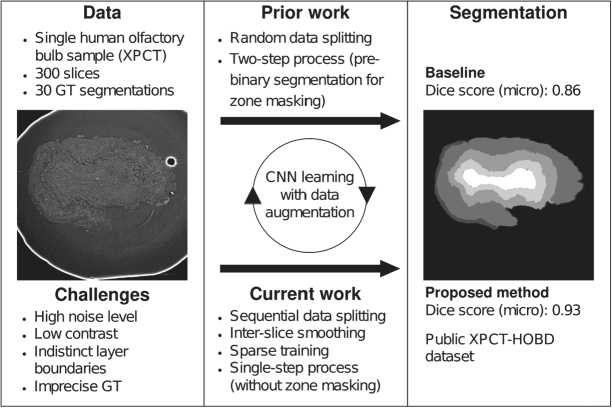
Fig. 1. Task and research outline

This article is organized as follows. The "Materials and Methods" section describes the data used, baseline approach, proposed methodology, and the ablation study conducted. The "Discussion" section is devoted to the analysis of the results obtained. The "Conclusion" section summarizes the paper.

Materials and Methods

Data description

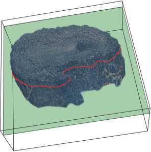
For the XPCT procedure, the OB sample was preliminarily fixed in formalin, then dehydrated and embedded in paraffin blocks. Then the sample was imaged using XPCT, resulting in a series of 2461 X 2461 2D tomographic slices [13]. We denote the original dataset, presented in paper [13], as D = {S i } f ₌₁, comprising N consecutive slices S t of the single OB sample. Fig. 2 a shows a 3D visualization ofthe OB volume, which we created by stacking N = 300 sequential tomographic slices using the Vedo framework [16].

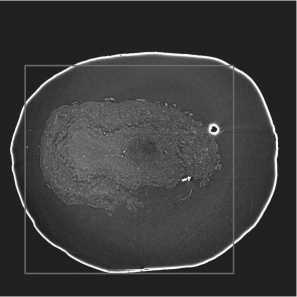
To decrease computational complexity and training time, expert-defined 864 X 864 regions of interest (ROIs) were extracted from each slice and used for model learning. An example of a slice with overlaid ROI is demonstrated in fig. 2 b .

a)

Fig. 2. Visualization: (a) 3D-volume of the OB from 300 consecutive slices; (b) OB slice with overlaid 864 X 864 ROI boundaries (purple)

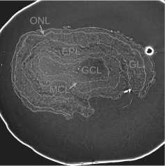
The OB has a multilayered morphology, including the olfactory nerve layer (ONL), glomerular layer (GL), external plexiform layer (EPL), mitral cell layer (MCL), and granule cell layer (GCL). Table 1 shows the distribution of pixel classes in the OB layers.

Tab. 1. The distribution of pixel classes for olfactory nerve layer (ONL), glomerular layer (GL), external plexiform layer (EPL), mitral cell layer (MCL), and granule cell layer (GCL), %

Id	Class	Median	Min	Max	Mean	Std
0	ground	66.69	64.18	69.74	66.92	1.61
1	ONL	3.13	1.51	4.37	2.99	0.76
2	GL	14.64	11.09	15.88	14.49	0.97
3	EPL	6.88	5.73	9.31	6.98	0.84
4	MCL	3.66	2.61	6.61	4.04	1.06
5	GCL	3.16	2.63	4.26	3.23	0.45
255	ignored	0.63	0.26	1.78	0.66	0.35

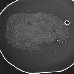
Fig. 3 a presents an example of the OB slice with the superimposed boundaries of these five layers. The bright white curve on the slice corresponds to the boundary between the paraffin and the surrounding air.

a)

b)

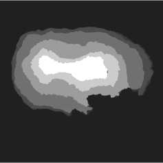
Fig. 3. Visualizations of the ROI example: (a) slice with layer boundaries; (b) the GT for this slice

GT includes five classes that correspond to the OB layers (see fig. 3 b ), as well as a background class labeled 0 and an "ignore" class labeled 255. For convenience, the OB layer classes are labeled from 1 to 5 towards the central OB layer.

Due to the indistinctness of the boundaries between layers on individual slices, GT for dataset D was made by the expert as follows. The initial dataset D splits into К = 30 non-intersecting chunks: D = Ц^ C i . Define the chunk C i = {S j } )=ioi-9 > i £ [1,30], S j £ D as ten consecutive slices.

For each chunk C_k , a synthetic image M i is obtained as an element-by-element inter-slice maximum intensity:

Mt (x, У) = max S,(x, y),

SjeCi where (x, y) denote the pixel coordinates.

GT G i was made based on M i and extended to all slices of the corresponding ten C_k . Thus, in addition to possible deviations of layer boundaries from the true layer boundaries, in general, GT made for the synthetic image M i may not correspond exactly to any slice in a chunk C i .

GT contains background pixels at the boundaries between layers, so such pixels have been replaced by an "ignore" class that is excluded from the calculation of the loss functions and quality score to avoid influencing the segmentation results.

The intensity values on the slices ranges from -1.15 X 10^-4 to 3 X 10^-3. However, the diagnostically significant information in the slices is concentrated within a narrow subrange of brightness. To isolate the relevant signal from the noise and artifacts, we performed a preliminary linear normalization of the intensity values /. The acceptable range was defined by expert-selected thresholds, with a lower bound L = 5 X 10^-4 and an upper bound U = 1.7 X 10^-3.

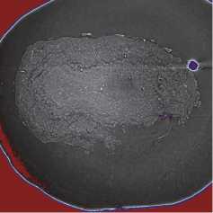
Analysis of the histogram in fig. 4 a indicates that most pixel intensities lie within the range [L, U]. The extreme values outside this range correspond to low-intensity noise at the bottom and high-intensity artifacts at the top, negative values have no physical meaning (see fig. 4 b ).

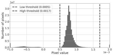
Fig. 4. (a) Histogram of the pixel distribution for 864 X 864 ROIs. The blue and red dashed lines mark the thresholds L and U, respectively; (b) Visualization of the OB slice showing pixels with intensity values below L in blue and above U in red

Intensity values beyond the range [L, U] were brought to the nearest boundary:

L, if I < L,

I' = j U, else if I > U, I,   otherwise.

The intensity values bounded by L and U were linearly normalized to the range [0,1] using the formula:

I =

I'-L

U-L'

To reduce the computational load, the slices and GT were compressed by half. Then, ROIs of 864 X 864 pixels were extracted from the central part of each.

Semantic segmentation quality assessment

The Dice score [17], which is widely used in image segmentation tasks, was chosen as the segmentation quality evaluation function. One of the key advantages of the Dice score is its robustness to the class imbalance observed in the dataset under consideration (see Table 1 in the subsection "Data description").

To obtain an overall assessment of the segmentation quality, a micro-averaged version of the Dice score was used [18], in which the quality is calculated without prior averaging at the individual class level. The Dice score with microaveraging is calculated as the harmonic mean of Precision_m / _cro and Recall_m / _cro with micro-averaging:

Precisionmlcro =

ZU TP /

ZU (TP/ + FP/)'

Recall

micro

Zt i TPj

ZU (TP / + FN / )'

^^ice micro

2 ■ Precision_micro ■ Recall_micro Precision micro + Recall micro '

where TP / , FP / and FN / are the numbers of true positive, false positive and false negative pixels corresponding to the i-th class.

Baseline training pipeline

The paper [13] describes a neural network model training pipeline for automated semantic segmentation of the OB layers using the U-Net [5] architecture.

The data were divided into training, validation, and test subsets randomly in the ratio of 240/30/30. To improve the model's generalization ability, the following augmentations were applied: random mirroring, rotation by a random angle from -90 to 90 degrees, and the addition of Gaussian noise with zero mean and standard deviation of 10 ~⁴ .

The training employed the RMSProp (Root Mean Square Propagation) optimizer with a momentum of 0.9. The learning rate was decreased by a factor of 10 whenever the validation metric stopped improving or the loss plateaued for two consecutive epochs. The authors used L2 regularization with "weight decay" of 10-8 and the batch size of 1.

The OB segmentation was performed in two steps. First, the OB was separated from the background with binary segmentation [13]. Next, the resulting binary segmentations (see fig. 5 b ) were applied to the original slices (see fig. 5 a ). Slices with masked backgrounds were passed to the model input for layer segmentation (see fig. 5 c ).

a)

b)

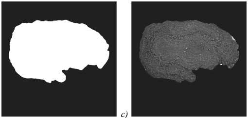
Fig. 5. OB masking: (a) ROI from the original slice; (b) OB binary mask; (c) masking result

Data splitting strategies

The dataset © is split into three disjoint subsets of slices:

V = ©i Ц ©г Ц ©'

where © i , D „ ,and V_t denote thetraining,validation,and test subsets,respectively, and N i = \V_i |, N_v = |B „ |' N_t = |V_t |.

Let define the data splitting strategies as S_r, S ^ , S_e and S_n, where n is the number of the starting validation chunk, n £N U {0}. S_r refers to a random split, where slices are assigned to training, validation, and test subsets randomly. S ^ , S_e, and S_n refer to sequential splitting strategies that are designed to minimize the number of pairs of adjacent slices from different subsets and isolate the slices of the test subset from those of the training subset. With sequential splitting, each subset consists of entire chunks: K_i chunks in the training subset, K_v in the validation subset, and K_t in the test subset, so that K = K_i + K_v + K_t = 30.

In the sequential splitting S_b, the test subset occupies the first K_t chunks of the volume, and the validation subset takes the next K_v chunks. The remaining K_; chunks are used for training.

S_n positions the test subset in the interior of the volume and surrounds it with two equal-sized validation parts, located immediately before and after the test subset. K_v is required to be even so that both validation parts contain the same number of chunks. All remaining chunks form the training subset.

S_e places the training subset at the beginning, followed by the validation subset, while the last K_t chunks are assigned to the test subset.

A formal description of data splitting strategies with a visualization is presented in Table 2.

Tab. 2. Data splitting strategies

Splitting	Visualization	Subsets
sr	^^^^Ш	H i = Random(D, Nt ) Dv = Random(D\Db Nv) D t = D\(D i U D „ )
S b		Di = Ui-Kt+K„ C i D v = U -^1 C i D t = ий ; 1 с -
Sn		Dr = (Ul^C i ) U (n^O n + Kv + Kt C j ) Dv = D\(Dt U D t ) г у 1on+| -Y\+Kt-1 D t = Il      к     С - J—t i-10n+\^\
S e		Di = U^ o 1 Ci D v = U^--1 C i D t = I"  C i i-K [ ^K -

Comparison of random and proposed sequential splitting strategies

To analyze the applicability of the strategy S_r used in [13], we trained two models with the same architecture and hyperparameters as described in the same work. The data were divided into training, validation, and test subsets according to strategies S_r and S_b.

Following the methodology from [13], we applied the reference OB binary masks, provided in the original publication, to mask the background on the original slices.

Fig. 6 shows plots of the Dice score dynamics for these models during training over 200 epochs.

a)

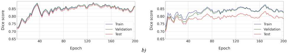
Fig. 6. Dynamics of the Dice score during model training with the pipeline from [13] using two data splitting strategies:

(a) Sr (random); (b) Sb (sequential, with the test subset located at the beginning of the volume)

The plots show that with S_r splitting (see fig. 6 a ), the quality scores for the training, validation, and test subsets are almost the same. In contrast, for S_b, the quality for the training and test subsets has significant differences (see fig. 6 b ), reflecting greater independence between subsets in sequential splitting. This independence makes S_b preferable to S_r .

The model trained according to the pipeline, described in [13], with S_b is used as the baseline in subsequent experiments.

The proposed training pipeline

In this paper, we propose a neural network training pipeline using S_b splitting into training, validation, and test subsets in the ratio of 240/30/30. A modified version of U-Net is used as the base architecture (see fig. 7).

The classical U-Net [5] architecture has a symmetric structure, including the downstream (encoder) and upstream (decoder) parts, between which information is transferred through connections between layers of the same level (skipconnections). In the proposed modification, each encoder block utilizes residual blocks with residual connections [19]

that bypass two convolutional layers within the block. Residual connections prevent gradient vanishing and improve information transfer from earlier layers.

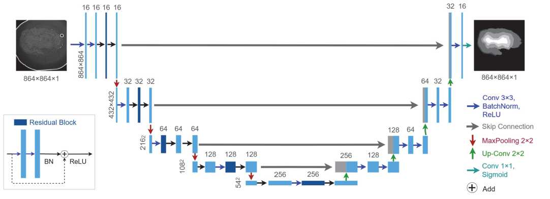
Fig. 7. Employed U-Net with residual blocks

During training, a fixed set of augmentations is applied to the "on-the-fly" data, including specular reflections, random rotations ranging from -180 to 180 degrees, and elastic deformations - random smoothed local pixel displacements that mimic natural variations in biological structures. The network parameters are optimized using the Adam algorithm with a 5 x 10 " ⁴ learning rate. Since a pronounced class imbalance characterizes the data, the focal loss function [20], which enhances the contribution of rare classes and reduces the influence of dominant classes, is chosen. The proposed pipeline assumes that the model is trained for 1000 epochs with a batch size of 2.

To reduce high-frequency noise, the original tomographic slices were preprocessed with inter-slice smoothing, which averages data using a sliding window size of 1 x 1 x 5.

Due to the visual similarity between neighboring slices, only the fourth and seventh slices from each chunk are used for training. These slices are separated by two intermediate slices, which reduces excessive correlation in the training subset. Segmentation quality assessment was performed on all slices, achieving a Dice (micro) score of 0.9325.

Class-specific Dice scores for the background and OB layers are presented in Tab. 3.

Tab. 3. Dice score for different data subsets and segmentation classes

Subset	Background	ONL	GL	EPL	MCL	GCL
train	0.993	0.936	0.975	0.954	0.943	0.972
validation	0.992	0.862	0.941	0.891	0.904	0.942
test	0.991	0.857	0.911	0.846	0.875	0.943

Analysis of subset order in sequential data splitting strategy

To evaluate the segmentation performance of the proposed pipeline relative to the baseline across different sequential data splitting strategies, we conducted experiments using a fixed training subset of 240 slices, a validation subset of 20 slices, and a test subset of 40 slices.

Tab. 4 compares the Dice Micro scores for the baseline and proposed pipelines across sequential splittings, with the last column (A) representing the difference between them.

The results demonstrate that, regardless of the specific sequential splitting strategy, the proposed pipeline consistently outperforms the baseline, yielding an improvement in the Dice score. Moreover, it shows greater robustness to the position of the test subset, as evidenced by the minimal variation in its performance. In contrast, the baseline model exhibits a high dependency on the test subset location, with its Dice score ranging from 0.754 to 0.942.

Ablation study

To evaluate the contribution of each improvement to the final segmentation quality, we conducted an ablation study comprising four experiments, each with one improvement removed from the proposed pipeline:

• 1.    OB pre-masking using reference binary masks.

• 2.    Training the model on initial slices, without prior inter-slice smoothing.

• 3.    Training the model on all slices from each chunk of the training subset. To ensure comparable weight updates when training on subsets of different sizes, the total number of epochs was proportionally adjusted to the size of the training subset. Using a full training subset, for example, training was conducted for 200 epochs.

• 4.    Training using a set of augmentations from the baseline.

All experiments used the S_b data splitting strategy.

Tab. 5 reports the Dice scores values for the baseline, the full proposed pipeline, and the training pipelines with one of the improvements disabled.

Tab. 4. Comparison of Dice Micro scores between the proposed and baseline pipelines across sequential data splitting strategies. Blue, green, and red correspond to the training, validation, and test subsets, respectively

	Sequential Splitting	Proposed	Baseline	A
S b		0.928	0.881	0.047
S00		0.940	0.908	0.032
S01		0.942	0.812	0.130
S02		0.937	0.927	0.010
S03		0.934	0.902	0.031
S04		0.929	0.919	0.011
S0S		0.931	0.901	0.029
S06		0.945	0.921	0.024
S07		0.938	0.909	0.030
S0R		0.938	0.897	0.042
S09		0.930	0.899	0.031
S10		0.935	0.754	0.181
S11		0.943	0.909	0.033
S12		0.947	0.840	0.107
S13		0.950	0.942	0.007
S14		0.950	0.941	0.009
S1S		0.948	0.893	0.055
S1fi		0.952	0.933	0.019
S17		0.952	0.923	0.030
S18		0.953	0.886	0.067
S19		0.952	0.908	0.044
S20		0.954	0.894	0.061
S21		0.960	0.841	0.119
S22		0.960	0.882	0.078
S23		0.961	0.826	0.135
S24		0.958	0.918	0.040
S e		0.957	0.830	0.127

Tab. 5. Ablation study results

Improvement	Baseline	Proposed	Exp. 1	Exp. 2	Exp. 3	Exp. 4
Pre-masking	✓	×	✓	×	×	×
Inter-slice smoothing	×	✓	✓	×	✓	✓
Sparse train	×	✓	✓	✓	×	✓
Alternative augmentations	×	✓	✓	✓	✓	×
Dice score (micro)	0.8620	0.9325	0.9159	0.9234	0.9164	0.9321

As shown in Tab. 5, the proposed improvements substantially enhanced the segmentation quality. Compared to the baseline, the Dice score increased from 0.8620 to 0.9325, an absolute gain of 0.07.

The largest decrease in quality occurred when the OB pre-masking step was omitted (Exp. 1), with Dice score dropping by 0.0166. This indicates that this step is optional in the proposed pipeline.

Training on the original slices (Exp. 2) results in a Dice score of 0.9234, confirming the importance of the data preprocessing step involving inter-slice smoothing. Including extreme slices from each chunk of the training subset, which weakly correspond to GT (Exp. 3), reduces the segmentation quality to 0.9164, a decrease of 0.0161. Replacing the set of augmentations in Exp. 4 with ones from the baseline leads to a negligible decrease in the Dice score.

Thus, the proposed training pipeline enhances the segmentation quality over the baseline, with each improvement contributing to the final segmentation quality.

Discussion

In this study, we analyzed a single sample of the human olfactory bulb, which is described in detail in [13]. Due to the limited size and specificity of the dataset, many proven methods and techniques for improving the quality of neural network segmentation are either not suitable or require additional adaptation and tuning.

Promising directions for future research include selection of ROI size, refinement of the intensity normalization method, and comprehensive evaluation of subsets ordering in the sequential data splitting strategy.

A logical continuation of our work is a transition to 3D-segmentation neural networks [7], which have shown great progress in biomedical research in recent years. Typical implementations process input tensors of size 643 or larger, and the datasets contain tens or hundreds of different annotated volumes. For the present task, however, the volume of data is extremely limited, necessitating smaller and non-cubic input tensors.

The ablation study revealed that the proposed change to the set of augmentations does not significantly impact the final quality of semantic segmentation. This suggests that the typical computer vision augmentations [21] are unsuitable for this task, since the distortions are of a different nature. The results indicate that the selection of relevant augmentations for this domain remains an open question.

A manual error analysis showed that the quality of the segmentation decreases for the initial and final slices in the chunks compared to the quality indicators for the central slices. The errors are localized mainly on the inner boundaries of the layers. This observation can be explained by the fact that, in the implemented method of obtaining the GT, the boundaries between layers change dramatically between successive slices in neighboring chunks (see fig. 8).

a)

b)

c)

Fig. 8. Visualization of GT segmentation: (a) the GT for slice S_2So; (b) the GT for slice S_2S1; (c) the difference map for slices S₂ so and S_2S1, where colored regions highlight mismatches (red - unique to slice S_2So, blue - unique to slice S_2S1}

This effect can be mitigated by using an enhanced annotation protocol that incorporates an ignore class. Such modification enables experts to explicitly label regions as belonging to specific OB layers or as representing areas of uncertainty. This scheme more accurately corresponds to the nature of the object under study, since there are no clear boundaries between the layers.

Another promising research direction is organizing a pipeline for the iterative improvement of the GT segmentation. This can be achieved by adapting existing interactive segmentation methods to the specific data type or by involving a human in the process and providing them with visual cues on the model's confidence levels. To improve the quality of segmentation, a refined geometric model of the object can be used in the form of restrictions on the shape of spatial boundaries between layers. Violations of such restrictions may provide additional clues for expert review. One more point to consider is the development of an alternative approach for evaluation methods that do not require the use of GT.

In the long term, improving the method may involve integrating specialized layers. For instance, Hough layers [22] could efficiently extract OB layer boundaries from XPCT images while significantly reducing the number of network parameters. Bipolar morphological layers [23, 24] could be used for computational optimization.

The released dataset and methodology facilitate the subsequent development of enhanced segmentation approaches for tomographic data segmentation.

Conclusion

This paper introduces an enhanced processing pipeline for semantic segmentation of human OB layers in XPCT reconstructions, building upon the approach from [13]. An important change in the training pipeline was revising the data splitting strategy to reduce the correlation between subsets for a more objective assessment of the segmentation quality. Unlike the pipeline mentioned above, the proposed pipeline uses a one-step approach to directly segment the OB layers without background masking. To account for the data’s unique characteristics, we propose preprocessing via inter-slice brightness smoothing and sparse training, using only central slices from each chunk in the training subset. The proposed training pipeline increases the test set's Dice score (micro) value from 0.86 (baseline) to 0.93. An ablation study showed that each of these changes contributes to this increase.

Data and code availability

The XPCT Human Olfactory Bulb Dataset (XPCT-HOBD), which includes raw slices and ground truth segmentations, has been published on Zenodo along with a pretrained neural network segmentation model and scripts for data preprocessing and inference, all freely available for download:

Ethics approval and consent to participate

The study was carried out on autopsy material obtained from the collection of the Avtsyn Research Institute of Human Morphology of the Federal State Budgetary Scientific Institution "Petrovsky National Research Centre of Surgery" (Moscow, Russian Federation). All protocols were approved by the Ethical Committee of the Research Institute of Human Morphology of the Russian Academy of Medical Sciences (now Avtsyn Research Institute of Human Morphology of Federal State Budgetary Scientific Institution "Petrovsky National Research Centre of Surgery") (No. 6A of October 19, 2009) and are in correspondence with instructions of the Declaration of Helsinki including points 7-10 for human material from 12.01.1996 with the last amendments from 19.12.2016.