Density-Based LLE Algorithm for Network Forensics Data

Published Online February 2011 in MECS

I INTRODUCE

With the enormous growth of computer networks usage and the huge increase in the number of applications running on top of it, network security is becoming increasingly more important. All the computer systems suffer from security vulnerabilities which are both technically difficult and economically costly to be solved by the manufacturers. Network forensics is the act of capturing, recording, and analyzing network audit trails in order to discover the source of security breaches or other information assurance problems. The term network forensics was introduced by the computer security expert Marcus Ranum in the early 90’s [1], and is borrowed from the legal and criminology fields where “forensics” pertains to the investigation of crimes.

According to Simson Garfinkel, network forensic systems can be implemented in two ways: “catch it as you can” and “stop look and listen” systems [2].

Most network forensic systems are based on audit trails. Systems relying on audit trails try to detect known attack patterns, deviations from normal behavior, or security policy violations. They also try to reduce large volumes of audit data to small volumes for interesting data. One of the main problems with these systems is the overhead, which can become unacceptably high. To analyze logs, the system must keep information regarding all the actions performed, which invariably results in huge amounts of data, requiring disk space and CPU resources. Next, the logs must be processed to convert them into a manageable format, and then compared with the set of recognized misuse and attack patterns to identify possible security violations. Further, the stored patterns need to be continually updated, which would normally involve human expertise. An intelligent, adaptable and cost-effective tool that is capable of this is the goal of the researchers in cyber forensics.

II Manifold Learning and KDDCUP’99 Data Set

• A.    KDD CUP’ 99 Data Set

  In 1998, the United States Defense Advanced Research Projects Agency (DARPA) funded an “Intrusion Detection Evaluation Program (IDEP)” administered by the Lincoln Laboratory at the Massachusetts Institute of Technology. The goal of this program was to build a data set that would help evaluate different intrusion detection systems (IDS) in order to

  assess their strengths and weaknesses. The objective was to survey and evaluate research in the field of intrusion detection. The computer network topology employed for the IDEP program involved two sub networks: an “inside” network consisting of victim machines and an “outside” network consisting of simulated real-world Internet traffic. The victim machines ran Linux, SunOS^TM, and Solaris^TM operating systems. Seven weeks of training data and two weeks of testing data were collected. Testing data contained a total of 38 attacks, 14 of which did not exist in the training data. This was done to facilitate the evaluation of potential IDSs with respect to their anomaly detection performance. Three kinds of data was collected: transmission control protocol (TCP) packets using the “tcpdump” utility, basic security module (BSM) audit records using the Sun SolarisTM BSM utility, and system file dumps. This data set is popularly known as DARPA 1998 data set [3].

One of the participants in the 1998 DARPA IDEP [4], used only TCP packets to build a processed version of the DARPA 1998 data set [3]. This data set, named in the literature as KDD intrusion detection data set [5], was used for the 1999 KDD Cup competition, which allowed participants to employ it for developing IDSs. Both training and testing data subsets cover four major attack ategories: Probing (information gathering attacks), Denial-of-Service (deny legitimate requests to a system), User-to-Root (unauthorized access to local super-user or root), and Remote-to-Local (unauthorized local access from a remote machine). Each record consists of 41 features [7], where 38 are numeric and 3 are symbolic, defined to characterize individual TCP sessions.

• B.    Manifold Learning

The articles in Science [7,8] proposed to recover a low-dimensional parameterization of high dimensional data by assuming that the data lie on a manifold M which, viewed as a Riemannian sub manifold of the ambient Euclidean space, is globally isometric to a convex subset of a low dimensional Euclidean space. This bold assumption has been surprisingly fruitful, although the extent to which it holds is not fully understood.

Each manifold learning algorithm attempts to preserve a different geometrical property of the underlying manifold. Local approaches (e.g. LLE [9], Laplacian Eigenmaps [10], LTSA [11]) aim to preserve the local geometry of the data. They are also called spectral methods, since the low dimensional embedding task is reduced to solving a sparse eigenvalue problem under the unit covariance constraint. However, due to this imposed constraint, the aspect ratio is lost and the global shape of the embedding data can not reflect the underlying manifold. In contrast, global approaches like Isomap [9] attempt to preserve metrics at all scales and therefore give a more faithful embedding.

• III Data Reduction

• A. Locally Linear Embedding Algorithm

The LLE algorithm is based on simple geometric intuitions. Suppose the data consist of N

→ real-valued vectors Xi , each of dimensionality D, sampled from some smooth underlying manifold. Provided there is sufficient data m(such that the manifold is well-sampled), we expect each data point and its neighbors to lie on or close to a locally linear patch of the manifold. We can characterize the local geometry of these patches by linear coefficients that reconstruct each data point from its neighbors. In the simplest formulation of LLE, one identifies k nearest neighbors per data point, as measured by Euclidean distance. The algorithm can be described as:

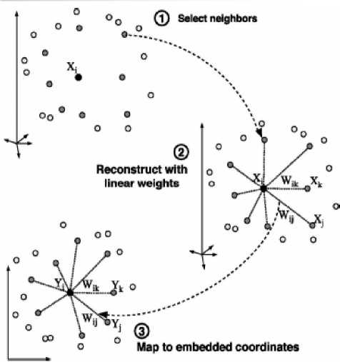
Fig 1 Locally Linear Embedding

• 1.    Find K nearest neighbors of each vector, X_i, in R^D as measured by Euclidean distance.

• 2.    Compute the weights W ij that best reconstruct Xi from its neighbors.

• 3.    Compute vectors Y_i in R^d reconstructed by the weights W_i j . Solve for all Y_i simultaneously.

Xi ~ У wx i j ij j

The algorithm can be described as Fig 1:

To compute the N x N weight matrix W we want to minimize the following cost function:

point is a measure of how sensitive its tangent line is to moving the point to other nearby points. There are a number of equivalent ways that this idea can be made precise.

One way is geometrical. It is natural to define the curvature of a straight line to be identically zero. The curvature of a circle of radius R should be large if R is small and small if R is large. Thus the curvature of a circle is defined to be the reciprocal of the radius:

^       ^

$ (W ) = Z x -£ , w , X j

i

R

Where W_i j =0 if X j is not one of the K nearest neighbors of X_i and the rows of the W sum to 1.

Z W«= 1                    (2)

The W like:

f0.3 0.2...)

W =

...       ... ...

Fig 2 show the relations of the Xi and his neighbors.

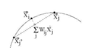
Fig 2 K nearest neighbors

At last, we get:

y = Z W j Y j              (3)

j

B Variable K-nearest neighbor LLE

In this section, we will introduce the key step in LLE, finding the k nearest neighbors. In traditional LLE algorithm, the k is invariable, which is suit for th e homogeneous distribution manifold. For the manifold flow, namely, the data is a flow and the distribution is heterogeneity, in order to remain the topology of the data, the k should be changed with the distribution.

Curvature is a good way to describe the changing of the manifold.

Let C be a plane curve (the precise technical assumptions are given below). The curvature of C at a

Given any curve C and a point P on it, there is a unique circle or line which most closely approximates the curve

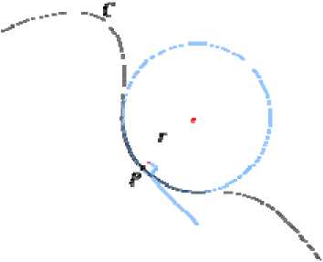
Fig 3 Curvature of the plane curve near P, the osculating circle at P. The curvature of C at P is then defined to be the curvature of that circle or line. The radius of curvature is defined as the reciprocal of the curvature.

Another way to understand the curvature is physical. Suppose that a particle moves along the curve with unit speed. Taking the time s as the parameter for C, this provides a natural parameterization for the curve. The unit tangent vector T (which is also the velocity vector, since the particle is moving with unit speed) also depends on time. The curvature is then the magnitude of the rate of change of T. Symbolically, k =

dT ds

For a plane curve given parametrically in Cartesian coordinates as γ(t) = (x(t),y(t)), the curvature is

k =

I ’ ”                  , ,,

xy - yx

x ²

Where primes refer to derivatives with respect to parameter t. The signed curvature k is(7)

For the less general case of a plane curve given explicitly as y = f(x) , and now using primes for derivatives with respect to coordinate x , the curvature is (8)

k =

, ,,                  , ,,

xy - yx

x ²

+ y’²

k=

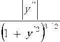
and the signed curvature is

k=

y

This quantity is common in physics and engineering; for example, in the equations of bending in beams, the 1D vibration of a tense string, approximations to the fluid flow around surfaces (in aeronautics), and the free surface boundary conditions in ocean waves. In such applications, the assumption is almost always made that the slope is small compared with unity, so that the approximation:

flow, the unchanged k cannot assure the topology of the local area.

Although, the curvature is a good way to describe the change of the curve, but with the increase the dimensions of the data, the curvature is not easy to get; in order to simple the process of guaranteeing the topology of the original data, a novel schema based density is introduced.

C Density based LLE

Analyzing the data, we use a simple way to replace the curvature, density around point c.

For a constant range around point p, we count the number of the instances of the range. The more instances indicated that the more complicated topology, namely, we should choose a greater K for point p in LLE algorithm. The algorithm of computing variable K-nearest neighbor can be described as:

Step 1 computing the mean density (MD) of whole dataset;

Step 2 given a nearest neighbors K and local range R;

Step 3 for point p in dataset d, we compute the density of p using range R(marked as LD),

Step 4 the variable K is:

Vk =

LD * K MD

d 2y

dx2

For a parametrically defined space curve in three-dimensions given in Cartesian coordinates by γ(t) =

(x(t),y(t),z(t)), the curvature is k =

(, z y - y z )² + (x z - z x )^z + ( y x - x y )² (11)

/2

From the definition of curvature, we can see that, the greater of k, the more complicated of the topology, namely, for point of curve C(marked as p), if the curvature of p is greater, we can get that the topology of points around p is complicated.

In traditional LLE algorithm, for very point in manifold, the k is unchanged. The schema didn’t considered change of the manifold. If the points of manifold are homogenous, the unchanged k will get a good result. But for the heterogen- eity distribution data

IV Data reduction

In this section, we reduce the data using the normal LLE and variable k LLE;

A Data Processing of the Data Set

In section 2, we know that each record of the Data set consists of 41 features where 38 are numeric and 3 are symbolic, at the same time, the dimension of each features are different. For example, the follow is a normal                                        record:

0,tcp,http,SF,181,5450,0,0,0,0,0,1,0,0,0,0,0,0,0,0,0,0,8,8, 0.00,0.00,0.00,0.00,1.00,0.00,0.00,9,9,1.00,0.00,0.11,0.0 0,0.00,0.00,0.00,0.00.

The first feature is “Length (# of seconds) of the connection”, the fifth feature is “data bytes from source to destination”, the seventh feature is a flag that “1 if connection is from/to the same host/port; 0 otherwise”. In order to find the attack data in the data set, we should apply the clustering algorithm on the data set. Before clustering, we must pre-process the data set:

• 1    Replacing the Symbolic with Numeric

The Fig2(Type of the protocol, e.g. tcp, udp, etc.),feature 3(Network service on the destination, e.g., http, telnet, etc.), feature 4(Normal or error status of the connection) features of the record are symbolic, there are three type of the protocol, 66 type of network service and 11 type of status in the data set. A simple way is used to replace the symbolic, 1 replace “tcp”, 2 replace “udp” and 3 replace “icmp”. the next 2 features with the same way. So we get the numerical record:

0,1,21,10,181,5450,0,0,0,0,0,1,0,0,0,0,0,0,0,0,0,0,8,8,0.0 0,0.00,0.00,0.00,1.00,0.00,0.00,9,9,1.00,0.00,0.11,0.00,0. 00,0.00,0.00,0.00.

• 2    Standardizing the Data Set

In the data set, the value of sixth features is much larger than the value of the second feature, which will affect the clustering, so we should eliminate the effect of the dimension.

x.(k) = Xi( k) - E (x( k))i        [var{x(k)}]1/2

Formula (4) is a way to standardize the data set, which make the average is zero and the variance is one. With the (4), we can get the record: -0.0354,-0.7746,0.7746,0,-0.3502,0.5836,0,0,0,-0.0614,0 ,0.7746,0,-0.0354,0,0,0,0,0,0,0,0,-0.8880,-0.9775,-0.077 2,-0.0765,0,0,0,0,-0.3165,-1.3338,-28.2666,0,0,-0.5937,0.4939,-0.1131,-0.2107.

• B . Data Reduction with LLE

With the previous works, we can get the algorithm of data reduction. The algorithm described as follow:

Input: Dataset S n×D , number of neighbors K, dimension of reduction d

Output: Dataset of reduction Y

Step 1: replaces the symbolic with numeric in Dataset S;

Step 2: standardizing the Dataset S with (12);

Step3: Computing reconstruction weights, for each point xi in S, set

Wt =

У C 7*

k jk

У C -1

lm lm

Step4: Compute the low-dimensional embedding.

• • Let U be the matrix whose columns are the eigenvectors of (I - W)^T (I - W) with nonzero

accompanying eigenvalues.

• • Return Y: = [U]n×d.

C Data Reduct on w th Var able K LLE

The variable K LLE can improve the effect of changing topology. The algorithm can be described as:

Input: Dataset S n×D , Mean number of neighbors K, dimension of reduction d

Step 1: replaces the symbolic with numeric in Dataset S;

Step 2: standardizing the Dataset S with (12);

Step 3: computing the Mean density of the DataSet;

Step3: Computing reconstruction weights, for each point xi in S, set

W =

У C 7*

k jk

У C ^{- 1}

lm lm

Step4: Compute the low-dimensional embedding.

• •    Let U be the matrix whose columns are the eigenvectors of (I - W)^T (I - W) with nonzero accompanying eigenvalues.

• •    Return Y: = [U]n×d.

IV Experiment and Results

In order to test the validity of the reduction, the clustering algorithm is used to analyze the original data set and the reduction dataset.

We extract part records of DoS,PROBE,R2L,U2R and NORMAL in the data set from original dataset randomly, 5 test dataset were gotten, namely, NORMAL and DoS, NORMAL and PROBE, NORMAL and R2L,

NORMAL and U2R, DoS,PROBE,R2L,U2R and NORMAL, each dataset contain 11204 records.

• A.    Evaluat ng Standard

There are 5 targets for the test, rate of reduction (RoR), time of decting (ToD), true positive rate(TPR), false positive rate(FPR) and omission rate(OR)

s ze of reduct on

RoR =----------- total s ze detected true attack records

TPR =-------------------- total num false attack records

FPR=--------------- total num true attack records but d d not detected

OR =---------------------------

total num

There are two parameters in the test are changed, the nearest neighbors K and the dimension of reduction d.

• B.    Test Result

30

3

35

4

40

5.25

50

7.61

60

10.88

70

13.55

35

99.6

1.8

0.4

40

99

3.4

1

50

98.8

1.8

1.2

60

98.8

3.2

1.2

70

98.6

3

1.4

7/41

30

97.4

0.2

2.6

35

98.8

1.4

1.2

40

98.4

2.2

1.6

50

98.8

2

1.2

60

96.8

2.8

3.2

70

96.8

3

3.2

8/41

30

95.2

0

4.8

35

96.8

2

3.2

40

96.2

2

3.8

50

97.4

2

2.6

60

96.8

2.2

3.2

70

95.6

2.2

4.4

We use the win 7 and the CPU is Intel(R) Core(TM) i5 2.40gHz, the computer is Dell.

At first, we use the schema introduced in section 3 to reduce the dimensional for the data set. With the experiments, we chose 30,35,40,50,60,70 as the nearest neighbors, the time consume is show in table 1.

Table 1 Reduction Time nearest neighbors Reduction Time(S) K

When we got the reduction data, we use the Fuzzy c-means (FCM) to cluster the data. We apply the FCM on the data set of NORMAL and DoS, NORMAL and PROBE. Fig 3-6 is the result of the experiment.

Table 2 the result of the data reduction

RoR	K	TPR(%)	FPR(%)	OR(%)
3/41	30	100	1.8	0
	35	99.8	0	0.2
	40	100	3.8	0
	50	99.6	2.8	0.4
	60	99.6	2.8	0.6
	70	99.6	3.4	0.4
4/41	30	100	1	0
	35	99.8	2.8	0.2
	40	99.6	3.4	0.4
	50	99.4	2.8	0.6
	60	99.4	2.8	0.6
	70	99.6	3	0.4
5/41	30	99	0.6	1
	35	99.6	2.2	0.4
	40	99.6	3.2	0.4
	50	99	2.8	1
	60	98.6	3.2	1.4
	70	98.8	2.8	1.2
6/41	30	98.4	0.2	1.6

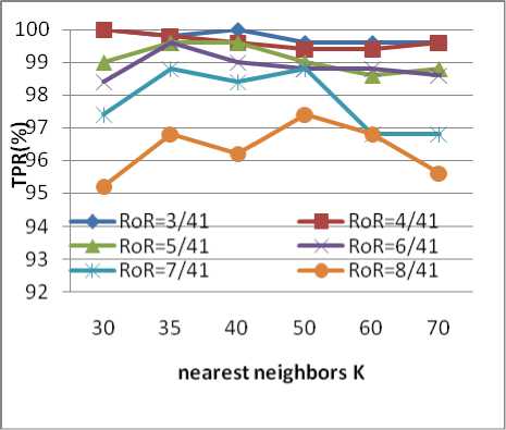
Fig 5 TPR of the DoS Attack

—♦—RoR=3/41 -e-RoR=4/41 —*-RoR=5/41

-r—RoR=6/41 —*—RoR=7/41 —e-RoR=8/41

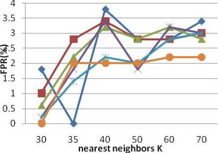
Fig 6 FPR of the DoS Attack

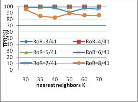
Fig 7 TPR of the Probe Attack

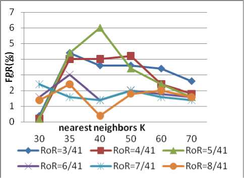
Fig 8 FPR of the Probe Attack

Fig 4 show that, for DoS attack, we can reduction 41 dimensional to 3 dimensional, which can assume the true positive rate more than 99%, and the reduction rate is 92.3%(1-3/41). With the increase the dimensional, the positive rate is decreased. Fig 5 show that the large reduction dimensional, the low false positive rate, Combining with Fig 3 and Fig 6, reducing the 41 dimensional to 4 is a good schema, which similarity to the schema proposed in[12].

Fig 7 shows that, for Probe Attack, when the dimensional reduced to 3,4,5,6 dimensional, the true positive rates are almost the same. Fig 8 shows that the large reduction dimensional, the low false positive rate. We can get that reducing the 41 dimensional to 6 is a best way, and the reduction rate is 85.36 %( 1-6/41).

V future work

Manifold learning is a good way to reduce the dimensional, especially, the manifold learning can maintain the topology of the data set, which can supply rich information for the data clustering, and the way is better than the schema using feature selection [12].

The LLE algorithm is a time consume way, the future work is to reduce the time consume.