Derivation and Implementation of the Collocation Methods for Solving Single and Multi Time-Fractional Order Differential Equations

The time-fractional differential equations have found extensive applications across multiple domains, including physics, mathematics, and engineering and these equations have been employed to model complex systems that exhibit anomalous diffusion or non-local behavior, which are characteristic of many physical processes, such as heat conduction in fractal materials, the dynamics of quantum systems, and the behavior of complex fluids. In such contexts, fractional models have provided deeper insights into the underlying mechanics, leading to more accurate predictions and a better understanding of the phenomena. Developing methods for solving fractional differential equations has expanded the mathematical toolkit available to researchers. Still, it has also led to new insights into the properties of these equations. The biosciences also benefit significantly from the application of fractional differential equations. For example, in the modeling of biological systems, such as the spread of infectious diseases or the dynamics of population growth, fractional models provide a more accurate representation of the processes involved. This is because many biological systems exhibit memory and hereditary effects, where the future state of the system depends not only on its current state but also on its history. Fractional models can capture these dependencies more effectively than traditional models [1, 2, 3].

In this paper, we focused our attention on the case of the single and multi-order time- fractional differential equations of the Caputo type as:

^^^(x) + (D^a,D ^a .....D))uW = f(x) x e [0,1]                 (1)

Subject to the conditions

и ⁽¹⁾ ( at) = ^сЛ = 1,2,3, .,⁽n-1),                                       (2)

Where D “ , D ^a , and D ^a are the fractional derivatives in the Caputo sense and a, P ,y (real or complex) are the order of the fractional derivative, ip is a constant, and f(x) is a continuous arbitrary smooth function.

The rest of the paper is organized as follows : Section 2 discusses related publications on fractional differential equations and the definition of fractional calculus. Section 3 presents the methodology employed for this research. Section 4 discusses convergence and error analysis. Section 5 discusses the numerical examples considered, and section 6 concludes the paper indicating future directions of the work.

2.    Related Works

In the last two decades, several analytical and numerical techniques have been developed to solve fractional differential equations, including [4] proposed and applied the Müntz-Legendre Tau method for solving fractional differential equations, [5] presented reproducing the kernel Hilbert space method to solve multi-order fractional differential equations, [6] employed optimization technique based on training artificial neural networks to solve fractional order differential equations, [7] generalizing the Lucas polynomial sequence approach for fractional differential equations, [8] applied effective modified Chebyshev differentiation matrices for fractional differential equations, [9] utilized the fractional backward differential formulas for fractional delay differential equations with periodic and anti-periodic conditions, [10] the homotopy analysis transform method was used to solve fractional order Riccati differential equation, [11] presented analytical approximate solutions of nonlinear fractional-order nonhomogeneous differential equations, [12] applied higher order methods for fractional differential equations based on the fractional backward differentiation formula of order three, [13] the fractional explicit Adams method was applied to solve fractional differential equations, [14] obtained numerical solution of the multi-order fractional differential equation using the Legendre wavelets and eigen function approach, [15] studied multi-order fractional differential equations with constant and variable coefficients, and [16] applied Adomian decomposition method for fractional time-Klein-Gordon equations using maple. The effective solution of fractional-order differential equations (FODEs) requires numerical methods that balance computational efficiency, accuracy, and adaptability to various problem domains. In this paper, the standard collocation method (SCM) and perturbed collocation method (PCM) were specifically chosen to reduce computational cost, more versatility, and applicability in solving time fractional-order differential equations.

• 2.1    Definition of relevant terms

Some fundamental definitions of fractional calculus are provided in this section. The following are some definitions attributed to Riemann-Liouville and Caputo sense: [17, 18]

Definition 1

In fractional calculus arbitrary order (all real numbers and complex values) are differentiation and integration of 317

the form: D 2 , D 2 , D 2

Definition 2

Let и e L ² ([0, T]), The definition of the Riemann-Liouville fractional derivative (RLFD) is

^{Dau (x)} = ц^)^^о ^(x-t)n "“ " ^{1 u(t)d} ;’   ^-~<^a<                 ⁽³⁾

where n is the smallest number that is greater than or equal to α

Definition 3

Let и ∈ Н^п ([0, т ]), the Caputo fractional derivative (CFD) of и ( х ) is defined by

Where п =[ р ]+1.

Hence, we have the following properties:

D^u ( X )=-(^ ∫ г ( X ^- t ) ^^U ( t )⁽ п ⁾ dt ; Р >0

г1^ахР =    ⁽ £+1 ⁾   ( а+Р )

⎧      = ( а+р+1 ₎        ,

J^aD^af ( х )= f ( X ); X >0

D^aC =0, С is a constant

⎪ D^ax^v =   ⁽ y+l ⁾ -x ( ■'—a )

⎩            = ( '-a+1 )        ^,

Where [ a ] denotes the smallest number that greater than or equal to a .

• 3.    Construction of orthogonal polynomials

• 3.1    Construction of orthogonal polynomial bases:

In this paper, an orthogonal polynomial was constructed and used as a basis function for solving the form equations (1) and (2). Orthogonal polynomials form a set of orthogonal functions concerning a weight function over a specific interval. It presents a promising alternative due to its ability to approximate functions and their derivatives efficiently. By representing both the differential and integral components in terms of orthogonal polynomial series [21].

The orthogonal polynomial on the interval [-1,1] was constructed using a set of the following equations

(            do ( x )= ^aoo

⎪        ( x )=Яц + ^awdo ( x )

q2 (X)=a22*2 + a21dl (X)+a2odo(X )

⎩⋮

Hence, using the orthogonality properties defined by

< Qn , Qm >=∫dn (X) Qm (X) dx =0,if n≠m(7)

and

< Qn, Qm >=∫) Qn (X) Qm (X) dx=0,ifn=

To compute Q 0( x ) goes thus,

⎧ < do ^, do >=1 ⇒ ∫ do ( x ) Qo ( X ) dx =1

⎪

∫ dx =    [x]ii=1

-1

V

2 a 00=1 ⇒ , doo ⁼ √2

Thus, the

1 do (x)=,

√2

Similarly, we computed Q 1( x ) as follows Here, we used the properties of orthogonality,

< <7o , <7i >=0

< <7o , <7i>=1   ( Ort ℎ onormal )

{

From (9), we have

⎧ ^<<7о ^,<7i >= ∫ ^Qo(х) ∗ <7i ( х ) dx =∫ _± «оо ( ^11^ ⁺ «io<7o ( x )) dx =0

к

∫ \ ^ = . ^11^ ⁺ «10 - / dx =0, ∫ \ 72 ^11 ^^+∫4 «10 ₂ d-X =0, ∫ * xdx + £10 ∫ dx =0,

√2’ J-1           2                ,

Implies «10 =0, From (10), we have

< <71 , <7i >=

∫ <71 (x) ∗ <71 (x) dx =∫ [^'11^' + «ю<7о (x)] ²dx =1

∫[ ^'11^' +0 Q о(X)] ²dx =1, sItics d^Q =0,

v

∫ [^'11'^'] ²dx =1,

an ∫ [ x ] ²dx =1,

⇒   =

,

<7i ( х )=

Thus, in general Qn ( X )=

^n ( X ), where ^n ( X ) a polynomial of degree n and is called Legendre polynomial

Pn ⁽ X )= 2ⁿn ! dx^{n (} x"-1)

This process is continued as follows:

(

2 (X)= ^√ Г (3X²-1), 4

<7з ⁽x)=√ \ ^.   2  /,

4 з

Qt ( x )=_√ .

'35x4-30x2 + 3\

.       8       /,

( 63x^s-70x³+15x )√ 22

⁽ 231X⁶-315x⁴+105x²-5 )√ 26

⎪ Q& ⁽ x ₎₌

⎩ _⋮

In this paper, the types of problems considered are defined on the interval [0,1]. To address this, we need to convert the orthogonal polynomials from the interval [-1,1] to [0,1]. Therefore, we first carry out the conversion of orthogonal polynomials from the interval [-1,1] to a general interval[ a , b ], and then specialize to the interval [0,1].

In this case, the linear transformation

X ∗₌ a^x + bi

Here, from [-1,1] to [ a , b ],

Suppose =-1,and x∗=a,x=1,and x∗=b, These resulted in the following system of equations га=-аг + bi                                        (18)

^{ b =   + bi                                            (19)

Solving (18) and (19) yields

{

( Ь—а )

О1 2

U —⁽ а+Ь ⁾

Substituting (20) and (21) into (17) we have,

∗ ⁽ Ь—а )( а+Ь )

2            2

From (22) after simplifying give

_∗ — ^2Х“ ( Ь+а ) = ₍ Ь—а )

Also, to convert from [-1,1] to [0,1], Here a=0, b=1. Hence (20) becomes,

X ^∗ =2 X -1

Substituting X ^∗ =2 X -1 into the constructed orthogonal polynomial (16) yields the orthogonal polynomials on the intervals of [0,1]

q₀ ( X _{)=  ,}

Qi (X)=√6X -√ , q2 (X) =3√10х2 - 3√10х+ | √10, q3 (х) =10√7х3 - 15√7х2 +6√7х- | √7,

q₄ ( X ) =105√2 х⁴ - 210√2 х³ + 135√7 х² - 30√2 X +I √2,

⎪        ( ) = 126√22  - 315√22  + 280√22  - 105√22  + 15√22 - √22,

⎪  ( ) = 462√26  - 1386√26  + 1575√26  - 840√26  + 210√26  - 21√26 + √26

⎩⋮

• 3.2 Description of proposed methods

• 3.2.1    Standard collocation method on fractional differential equation (SCM)

In this work, two types of collocation methods are proposed which are known as the standard collocation method (SCM) and the perturbed collocation method (PCM). These methods are demonstrated on the fractional order differential equations (1) and (2) as follows:

We consider the fractional order differential equation of the form:

∑1=0 Pt ( X ) и¹ ( X )+( D^a , DP ,…, D^ ) и ( X )= f ( X ),   X ∈ [0.1]                       (26)

Subject to the conditions

и ⁽¹ ) ₍ a_t )= ^i ; i =1,2,3,…,( n -1),                                   (27)

(26) can be expanded as

Pa ( x ) и ( X )+ Pl ( X ) и / ₍ X )+ P₂ ( X ) и // ₍ X )+ ⋯ + ^n ( X ) uⁿ ( X )+( D^a , DP …, D^Y ) и ( X )= f ( X )       (28)

Let's assume an approximate solution of the form:

U_N ( X )=∑ i=₀CtQt ( X )

Where N is the computational length and substitute (29) into (28) to get

Po (x) Un (x)+Pi (X) uN /( X)+p2 (X) uN //( X)+⋯+^n (X)uNn (X)+(Da, DP …,W) uN (x)=f(x)

• (29)    can be expanded as

UN (X)=coQo(x)+CiQi(X)+C2Q2(X)+⋯+cnQn (X)

Substitute (31) into (30) to get

(      p₀ ( X )( ^coQo ( X )+ ^ciQi ( X )+ C₂Q₂ ( X )+ ⋯ + ^cnQn ( X ))+

Pl ( X )( ^coQo / ₍ X )+ C1Q1 / ₍ X )+ ^c₂Q₂ / ₍ X )+ ⋯ + ^cnQn / ₍ X ))+

.    P2 (X)(coQo //( X)+C1Q1 //( X)+c2Q2 //( X)+⋯+cnQn //( X))+

⎪      ^n ( X ₎ ⋮ ₍ c_oQo^l ( X ) + C1Q1¹ ( X _{) +} c₂Q₂ⁿ ₍ X )+ ⋯ + CnQn¹¹ ( x ))+

⎩ ( D^a , DP …, DY )( ^coQo ( X )+ ^ciQi ( x )+ c₂Q₂ ( X )+ ⋯ + ^cnQn ( x ))+ f ( x )

Hence, collecting like terms in (32) to get

• ⎧    c₀ ( Po ( x ) Qo ( x )+ Pi ( X ) Qo / ₍ x )+ P₂ ( X ) Qo // ₍ x )+ ⋯ + ^n ( X ) Qo ⁽ n ) ₍ X )+( D^a , DP …, DY ) Qo ( x ))+

⎪^⎪     Cl ( Po ( X ) Qi ( X )+ Pl ( X ) Q1 / ₍ X )+ p₂ ( X ) Q1 // ₍ X )+ ⋯ + ^n ( X ) Qi ⁽ n ) ₍ X )+( D" , DP …, DY ) Qi ( X ))+

• ⎪^{⎪⎨      (} '• ⁽■^)&(■ )+ ' ⁽■⁾. / ( ■ )+ '■ ⁽ ■ ⁾. // ( ■ )+_⋮ ⋯ +.⁽■⁾t ⁽ ) ( ■ )+( , ^,   …, . ⁾.⁽■ ))+    (33)

⎩^{⎪ C}N ( Po ( X ) Qn ( X )+ Pl ( X ) Qn / ₍ x )+ P₂ ( X ) Qn // ₍ x )+ ⋯ + ^n ( X ) Qn ⁽ " ) ₍ x )+( D^a , DP …, DY ) Qn ( X ))+ f ( X )

Thus (33) gives (N+1) unknown constants ( ^ci ; i ≥0) to be determined. Consider the initial conditions given in equation (27), we obtain

( u_N ( a_r )= Фо ⇒ CqQo ( a_r )+ ciQi ( a_r )+ c₂Q₂ ( a_r )+ ⋯ + ^cnQn ( a_r )= Фо , (34) ⎪ и ^/ N (^ai)= Ф1 ⇒ CoQ ^/о (^ai)+ CiQ ^/ , ( a₁)+ c₂Q ^/₂( a₁)+ ⋯ + CnQ ^/ N (^ai)= Ф1 , (35) ■и // N (^ai)= ф₂ ⇒ CoQ // о (^ai)+ CiQ // , (^ai)+ c₂Q // ₂ (^ai)+ ⋯ + ^cnQ // N (^ai)= ф₂ , (36)

⎩ и ⁽ п-1 ⁾ N ( di )= Ф (n-1) ^⇒ CoQ ( n-1 ⁾о ₍ a_{r ) +} CiQ ⁽ n-1 ⁾ , ( a_{r ) +} c₂Q ₍ n-1 ⁾ _{2 (} a_r )+ ⋯ + ^cnQ ( n-1 ⁾ N ( a_{r ) =} Ф (n-1), (37)

(

Thus, equation (33) is then collocated at point X = to get,

Co ( Po ( ^xk ) Qo ( ^xk )+ Pl ( ^xk ) Qo / ₍ ^xk )+ p₂ ( ^xk ) Qo // ₍ ^xk )+ ⋯ + ^n ( ^xk ) Qo ⁽ n ) ₍ ^xk )+( D^a , DP …, DY ) Qo ( ^xk ))+

Cl ( Po (xk ) Qi (xk)+Pl (xk ) Qi /( *k)+p2 (xk ) Qi //( Xk)+⋯+^П (xk) Qi (n)( Xk)+(Da, DP …,DY ) Q1 (xk))+ c2 ( Po (xk) q2 (xk)+Pl (xk ) q2 /( xk)+p2 (xk) q2 //( X)+⋯+^n (xk ) q2 (n)( xk)+(D", DP …,DY ) Q2 (xk ))+    (38)

⎩^{⎪ C}N ( Po ( ^xk ) Qn ( ^xk )+ Pl ( ^xk ) Qn / ₍ ^xk )+ p₂ ( ^xk ) Qn // ₍ ^xk )+ ⋯ + ^n ( ^xk ) Qn ^{( 1} ) ₍ ^xk )+( D^a , DP …, DY ) Qn ( ^xk ))+ f ( ^xk ),

Where,

Xk =  + ⁽ s ⁾ I ; к =1,2,3,…,( N ^- n +1) ,

An algebraic linear system of equations in ( N +1) unknown constants is thus obtained from (38) for ( N - n +1). Additional n equations are derived from equations (34) to (37). Altogether, (N+1) algebraic equations in (N+1) unknown constants are determined, and the unknown constants are obtained by using the Gaussian elimination approach, and the results obtained and substituted back into equation (29) to get the required approximate solution.

• 3.2.2 Perturbed collocation method on fractional differential equation (PCM)

Slightly perturbed (28) from the previous sub-section 3.2.1 and get

(P_Q (x)u_N(x) + P₁(x)u_N^/(x) + P₂(x)u_N^//(x) + — + P_n(x)u_Nⁿ(x) + (D “ ,D P ...,D^Y)uN(x)=f(x) + ^TjQN-_{n +} j (x)

7 = 1

Substitute (31) into (39) to get

"            P_o C0( C_OQ_OM + CrQ^x) + CqQ₂(x) + — + C n Q n CO) +

P l W(c₀Q o/ (x) + qQ /(x) + C 2 Q 2 /(x) + — + C n Qn^x)) +

, P2(x)( CoQo//(x) + CiQ i//(x) + C2Q 2 //(x) + — + CnQn//(x)) +(40)

• P _n (x)(c₀ Qo ”(x) + c, Q. ⁿ(x) + C 2 &  ⁿ(x) + — + c_n Q_nⁿ (x)) +

l(D “ ,D P ...,D ^ )(C o Q o (x) + C i Q i (x) + C 2 Q 2W + — + C N Q N (x))+f(x) +Z 7= ^ Q n (x)

Hence, collecting like terms in (40) to get

Co (Po(x)Q o(x) + Pi(x)QoZ(x) + P2(x)Qo/Z(x) + — + Pn(x) Q o(n)(x) + (D “,D P ...,Dy)Qo(x))+

Ci (Po(x)Q i(x) + Pi(x)Q/(x) + P2(x)Q//(x) + — + Pn(x) Q i(n)(x) + (D “,D P ...,D^)Qi(x))+

C2 (Po(x)Q 2(x) + Pi(x)Q2 /(x) + P2(x)Q2 "(x) + — + Pn(x) Q 2(n)(x) + (D “,D P .,D^(x))+

:(41)

C n (P o (x)Q n (x) + P i (x)Q n^/ (x) + P 2 (x)Q n^// (x) + — + P_n(x) Q N⁽ⁿ⁾ (x) + (D “ ,D P .,D ^ )Q n (x)) +

к

^{f (x)} +^k^Q n - n+j ^(x) 7=1

Thus (41) gives (N+1) unknown constants (c; i >  0,T j ; j >0 ) to be determined. Consider the initial conditions given in equation (27), we obtain,

" U_N (d i ) = V o ^ C o N o (O i ) + C i Q i (d i ) + C 2 Q 2 ⁽d i ) + — + C N Q N^i ) = V o , u /N^i ) = V i ^ C o Q ^(dj + C i Q / _i⁽d i ⁾ + C 2 Q /-/di ) + — + C n Q ^(d i ) = V) i ,

+ #

• ⁴ u "nCo i ) = V 2 ^ C o Q "ofaO + C i Q // /dj + c - Q "^dj + — + C n Q //^i) = V 2 ,

• (n- ^(аО^п-i) ^ Co Q^- Ц _о(_й1 ) + Ci Q⁽"- 4 ^ ) + c₂ Q^~ ^ ₂(di) + — + c_NQ^~ « ^d, ) = ^ - ^

Thus, (41) is then collocated at point x = x_k to get

C o (P o (x_fc)Q o (x_fc) + P i (x_fc) Q o^/ (x_fc) + P-fe) Q o^// (x_fc) + — + P n (x_fc)Q o⁽ⁿ⁾ (x_fc) + (D “ ,D P ...,D^Q o (x_fc)) C i (P o(x _fc)Q i (x_fc) + P i (x_fc) Q i^/ (x_fc) + P-fe)Q i^// (x_fc) + — + P_n(x_k) Q i⁽ⁿ⁾ (x_fc) + (D “ ,D P .,D^Q i(x _fc)) C 2 (P o (x_fc)Q 2 (x_fc) + P i (x_fc) Q -/ (xj + P 2 (x_fc)Q 2 "(x) + — + P n (x_fc)Q 2⁽ⁿ⁾ (x_fc) + (D “ ,D P .,D ^(xj)

+

+

+

C n (P o (x_fc)Q N (x_fc) + P i (x_fc)Q N^/ (x_fc) + P 2 (x_fc)Q N^// (x_fc) + — + P n (x_fc)Q N⁽ⁿ⁾ (x_fc) + (D “ ,D P .,D^ Q^xj)

к

Where

f (xj +^T j Q n -n+j (x_fc)

7 = 1

An algebraic linear system of equations in (N + 3) unknown constants is thus obtained from (46) for (N + 3). Additional n equations are derived from equations (42) to (45). Altogether, (N+3) algebraic equations in (N+3) unknown constants are determined, and the unknown constants are obtained by using the Gaussian elimination approach, and the results obtained and substituted back into equation (29) to get the required approximate solution.

4.    Convergence and Error Analysis

In this section, the convergence and error analysis of the proposed SCM and PCM on fractional order differential equations are discussed as follows:

• 4.1    Consistency: Define the residual R_N(x) as:

• 4.2    Stability:

Rn(%) = ^ 0 PiMu[(x) + (D fDP.....D))uN(x)-f(x)(47)

If u(x) is the exact solution, then.

RN(x==£pP)x№(x+D(Da,DP.....D^u^x--f(x) = 0

For u_N(x) to converge to u(x) as No o,R_N(x) converge to 0 uniformly on [ a, b ]: ||T?_N(x)|| ^ 0 as Nora

Stability is determined by the properties of the matrix of the linear system obtained from collocation

A c = b(49)

Where A is the matrix formed by evaluating the derivatives of basis functions and the fractional derivative term at the collocation points, c is the vector of coefficients {c_fc}, and b is the vector of f(x _fc).

Stability is ensured if the condition number of A remains bounded as Nora.

• 4.3    Uniqueness:

• 4.4    Error Analysis:

The linear system Ac = b has a unique solution if A is invertible. The invertibility of A is guaranteed if the basis functions Q ! (x) and the collocation points x_k are chosen appropriately.

The error

E N(x) = uN(x) - u(x)

depends on the smoothness of the exact solution ( ) and the completeness of the basis functions

IIM*)II = |Z^ oP(^ SvW + (D a, D ^.....D Y)uN(x)-f(x)\\(51)

The error is bounded by

|IM*)II

Where C is a constant dependent on the matrix properties and the problem domain.

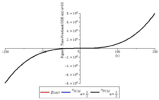
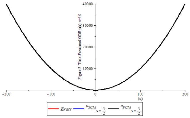
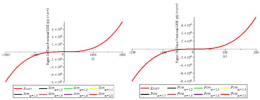
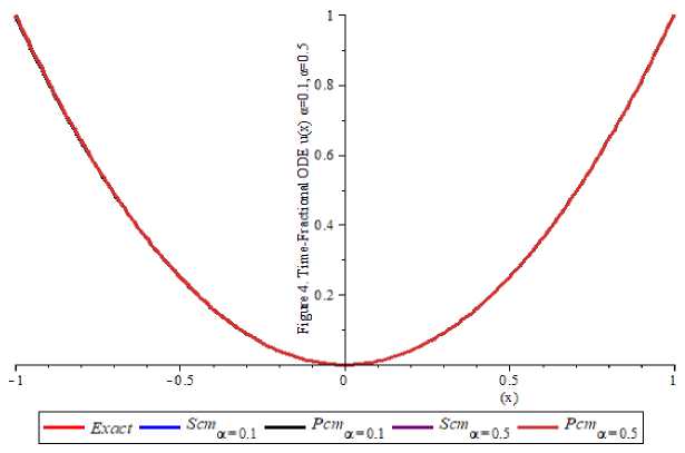
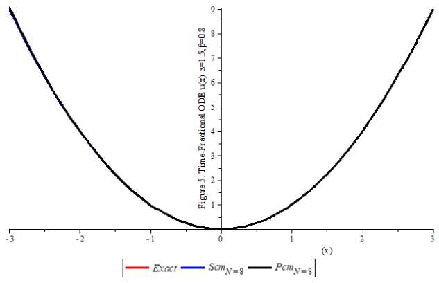
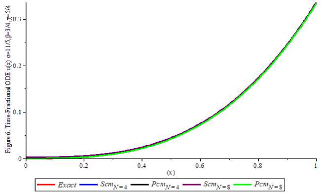
5.    Numerical Examples

This section presents six numerical examples to show the efficiency and feasibility of the proposed techniques. The first four examples are related to the single time-fractional orders while the last two are multi-fractional orders differential equations. The proposed standard collocation method (SCM) and perturbed collocation method (PCM) are employed for the two constructed orthogonal polynomials considered. In all examples, the Maple 18 software was employed to implement the numerical solutions of the test equations considered. The solutions are reported on the tabular forms and 2D plots are used to depict the numerical solutions for the six examples considered. See Appendix

Example 1 Consider the single-order time-fractional Bagley-Torvik equation which describes the motion of a rigid plate of the form [19]

D^au(x)+и //₍X)+и(X)=X(х² +√ + 6), X∈ [0,1]

, subject to the initial conditions: и(0) = и^/(0) = 0, ⎪ ₌3 “ ^{( 1} )= _⎩ for =

We applied the proposed methods SCM and PCM for the numerical solutions for example 1 at the best 3

computational length N=4. The numerical results for the а = were presented in Table 1 with the exact solution indicating that the proposed methods yield a good agreement with the numerical results presented in the literature [19]. The Figure 1. Depict the good agreement between the exact solution provided in equation (55) which shows the convergence of the а = equal to и(х)=х³ and the approximate solutions are presented for the N=4 as follows:

(и(    .) SCM≅ 9.00Е- 16- 2.10Е - 14х² + 1.0000000х³ - 5.213786081Е - 15х⁴

^{и(    . .₎РСМ≅ 1.60000Е - 15 + 3.60000Е - 13х² + 0.999999999х³ - 3.36515456X⁴

Table 1. Numerical solutions for Example 1 at the =

X	Exact solution	SCM	PCM	[19]
0.11	0.00133000000	0.0013310000000	0.0013200000000	0.0014942400000
0.16	0.00410000000	0.0040960000000	0.0041000000000	0.0043559100000
0.21	0.00930000000	0.0092610000000	0.0093000000000	0.0095516400000
0.26	0.01760000000	0.0175759999999	0.0176000000000	0.0177723900000
0.31	0.02980000000	0.0297909999999	0.0297999999999	0.0297080000000
0.36	0.04670000000	0.0466559999999	0.0467100000000	0.0460474300000
0.40	0.06400000000	0.0639999999999	0.0640000000000	0.0674789400000
0.45	0.09110000000	0.0911249999999	0.0911000000000	0.0946901600000
0.50	0.12500000000	0.1249999999999	0.1250000000000	0.1228509500000

Fig. 1. Numerical comparison solutions for Example 1

Example 2 Consider the single-order time-fractional Bagley-Torvik equation which describes the motion of a rigid plate of the form [19].

D^au(X)+и //₍X)+и(X)=2+X² + 4√ , X∈ [0,1]

у И subject to initial conditions:      и(0) = и/(0) = 0,

The exact solution of equations (57) and (58) is и(X)=X²

for а=.

We applied the proposed methods SCM and PCM for the numerical solutions for example 2 at the best computational length N=4. The numerical results for the a = were presented in Table 2 with the exact solution indicating that the proposed methods yield a good agreement with the numerical results presented in the literature [19]. The Figure 2. Depict the good agreement between the exact solution provided in equation (59) which shows the convergence of the a = equal to и(x)=x²and the approximate solutions are presented for the N=4 as follows:

(и( .) SCM≅ 8.359374E - 16 + 0.999999x² + 1.6404910E-14x³ - 6.561829499E-15x⁴ (60) ^{и( . )^.PCM≅4..46374E-16+2.00E-15x + 1.00x² - 2.27003E-13x³ + 1.1905139 - 13x⁴ (60)

Table 2. Numerical solutions for Example 2 at the =

X	Exact solution	SCM	PCM	[19]
0.1	0.01000000000	0.0100000000000007	0.0100000000000	0.010000001723771
0.2	0.04000000000	0.0400000000000004	0.0400000000000	0.040000046369413
0.3	0.09000000000	0.0899999999999999	0.0900000000000	0.090000089366190
0.4	0.16000000000	0.1600000000000000	0.1600000000000	0.160000120342059
0.5	0.25000000000	0.2500000000000000	0.2500000000000	0.250000148387098
0.6	0.36000000000	0.3599999999999990	0.3600000000000	0.360000175093239
0.7	0.49000000000	0.4899999999999990	0.4900000000000	0.490000200907060
0.8	0.64000000000	0.6399999999999980	0.6400000000000	0.640000225992179
0.9	0.81000000000	0.8099999999999980	0.8100000000000	0.810000250421551
1.0	1.00000000000	0.9999999999999930	1.0000000000000	1.000000273512726

Fig. 2. Numerical comparison solutions for Example 2

Example 3 Consider the single-order time-fractional order boundary value problem of the form [14]

⎧D^au(x)+и(X)= _-X^{3 a}-_-X^{2 a} + X² (X-1), X∈ [0,1] 1<a≤2 , (61) ⎪ Γ(4- ) Γ(3- )

subject to initial and boundary conditions: и(0) =0, и(1)=0 (62) ⎪ The exact solution of equations (61) and (62) is и(x)=x² (X-1) (63) ⎩for a = 1.2,1.3,1.4,1.5,1.6,1.8,2.0

We applied the proposed methods SCM and PCM for the numerical solutions for example 3 at the best computational length N=4. The numerical results for each of the a = 1.2,1.3,1.4,1.5,1.6,1.8,2.0 are presented in Table 3 with the exact solution indicating that the proposed methods yield a good agreement with the numerical results presented in the literature [14]. Figure 3a and Figure 3b depict the good agreement between the exact solution provided in equation (63) which shows the convergence of the a = 1.2,1.3,1.4,1.5,1.6,1.8,2.0 equal to и(x)=x² (x-1) and the approximate solutions are presented for the N=4 as follows:

и(   .) SCM≅ -1.0000E-10+4.190E-9x - 1.0000x² + 1.0000x³ - 8.0133E8x⁴

и(   . )^.SCM≅ -2.000E-11+4.2600E -9x - 1.0000x² + 1.0000x³ - 6.1594E-8x⁴

⎪и(   .) SCM≅ -3.000E-11+2.580E-9x - 1.00000x² + 1.00000X³ - 2.6566E8X⁴

■ и(   .) SCM≅ 4.0000E-11+3.670E -8x - 0.99999x² + 0.99999X³ + 3.0118E8X⁴      (64)

и(   .) SCM≅ 1.0000E-11-1.4500E8 - 0.99999x² + 0.9999x³ + 6.8457E-9x⁴

⎪и(   .) SCM≅ 1.101000E-7x - 0.9999999x² + 1.0000000x³ + 9.98473255E-9x⁴

⎩и(   . .₎SCM≅ 4.0000E-11-2.03E-9x - 1.00000x² + 1.00000x³ - 5.08625E -9x⁴

и(   .) PCM≅ 3.0000E-9+5.5E-9x - 1.00000x² + 0.99999X³ + 1.56204E8X⁴

и(   . )^.PCM≅ 5.0000E-11+1.4400E-8x - 1.00000x² + 0.99999X³ + 1.9453E8X⁴

⎪и(   .) PCM≅ 4.0000E-11+1.500E-8x - 1.00000x² + 1.00000x³ + 1.140519E9x⁴

■и(   .) PCM≅ 7.0000E-11-2.36000E-8x - 0.9999x² + 1.00000x³ - 1.89472E8x⁴ (65)

и(   .) PCM≅ -1.00000E-11-1.19E-8x - 0.9999x² + 1.000000x³ - 6.35310E9x⁴

⎪и(   .) PCM≅ 1.0000E-11-8.360E-8x - 1.00000x² + 1.000000X³ - 1.13556E7X⁴

⎩и(   .) PCM≅ 1.0000E-11-1.75E-8x - 1.00000x² + 1.000000X³ - 1.4200519E8X⁴

Table 3. Numerical solutions for Example 3 at the a = 1.2,1.3,1.4,1.5,1.6,1.8,2.0

X	Solutions	a=1.2	a=1.3	a=1.4	a=1.5	a=1.6	a=1.8	a=2.0
0.0	Exact	0.000000	0.000000	0.000000	0.000000	0.000000	0.000000	0.000000
	[14]	0.000000	0.000000	0.000000	0.000000	0.000000	0.000000	0.000000
	SCM	0.000000	0.000000	0.000000	0.000000	0.000000	0.000000	0.000000
	PCM	0.000000	0.000000	0.000000	0.000000	0.000000	0.000000	0.000000
0.2	Exact	-0.03200	-0.03200	-0.03200	-0.03200	-0.03200	-0.03200	-0.03200
	[14]	-0.03203	-0.03203	-0.03203	-0.03203	-0.03203	-0.03203	-0.03203
	SCM	-0.03200	-0.03200	-0.03200	-0.03200	-0.03200	-0.03200	-0.03200
	PCM	-0.03200	-0.03200	-0.03200	-0.03200	-0.03200	-0.03200	-0.03200
0.4	Exact	-0.09600	-0.09600	-0.09600	-0.09600	-0.09600	-0.09600	-0.09600
	[14]	-0.09607	-0.09607	-0.09607	-0.09607	-0.09607	-0.09607	-0.09607
	SCM	-0.09600	-0.09600	-0.09600	-0.09600	-0.09600	-0.09600	-0.09600
	PCM	-0.09600	-0.09600	-0.09600	-0.09600	-0.09600	-0.09600	-0.09600
0.6	Exact	-0.14400	-0.14400	-0.14400	-0.14400	-0.14400	-0.14400	-0.14400
	[14]	-0.14409	-0.14409	-0.14409	-0.14409	-0.14409	-0.14409	-0.14409
	SCM	-0.14400	-0.14400	-0.14400	-0.14400	-0.14400	-0.14400	-0.14400
	PCM	-0.14400	-0.14400	-0.14400	-0.14400	-0.14400	-0.14400	-0.14400
0.8	Exact	-0.12800	-0.12800	-0.12800	-0.12800	-0.12800	-0.12800	-0.12800
	[14]	-0.12810	-0.12810	-0.12810	-0.12810	-0.12810	-0.12810	-0.12810
	SCM	-0.12800	-0.12800	-0.12800	-0.12800	-0.12800	-0.12800	-0.12800
	PCM	-0.12800	-0.12800	-0.12800	-0.12800	-0.12800	-0.12800	-0.12800
1.0	Exact	0.000000	0.000000	0.000000	0.000000	0.000000	0.000000	0.000000
	[14]	0.000000	0.000000	0.000000	0.000000	0.000000	0.000000	0.000000
	SCM	0.000000	0.000000	0.000000	0.000000	0.000000	0.000000	0.000000
	PCM	0.000000	0.000000	0.000000	0.000000	0.000000	0.000000	0.000000

Fig. 3. Numerical comparison solutions for Example 3

Example 4 Consider the single-order time-fractional order initial value problem of the form [12, 20]

⎧ Dau(x)+и(X)=x2+(-)x2 “,  X ∈ [0,1](66)

⎪                            Γ(3 -)

subject to initial conditions:      и(0) = 0,(67)

⎪ The exact solution of equations (66) and (67) is и(X)=х2(68)

⎩ for а = 0.1 сстмИ ос = 0.5

We applied the proposed methods SCM and PCM for the numerical solutions for example 4.4 for the computational length N=8 is presented in Table 4 with the exact solution indicating that the proposed methods yield a good agreement with the numerical results presented in the literature [12, 20]. Figure 4 depicts the good agreement between the exact solution provided in equation (68) which indicates the convergence of the ос = 0.1 and ОС = 0.5 equal to и(X)=х² and the approximate solutions are presented for the N=8 as follows:

и(   .) SCM₈≅ 1.00Е - 10 - 3.00Е-9х+ х² - 1.412Е-8х³ - 2.7812Е-7х⁴ + 0.000001х⁵ +

-0.000000137х⁶ + 0.0000000102х⁷ - 7.65867Е -8х⁸

и(   .) РСМ₈≅3Е - 10 + 0.00001108Е-9х + 0.99х² + 0.0000018X³ - 0.000692X⁴ + 0.0014X⁵ +

-0.001678X6 + 0.001018888X7 - 0.0002517X8

и(   .) SCM₈≅2Е - 8 + 1.69Е-8х + 0.9х² + 0.000000019х³ - 0.000000076х⁴ + 0.0000173х⁵ +

-0.00002261х6 + 0.000001569х7 - 0.000000447х8

и(    .) РСМ₈≅ 2.0Е - 10 - 1.18Е-7х + 1.000004х² - 0.0000243X³ + 0.00008X⁴ - 0.00015X⁵ +

0.00002427X6 - 0.00007524X7 + 0.00001525X8

Table 4. Numerical solutions for Example 4 at the а = 0.1 and а = 0.5

X	Exact		SCM	PCM
0.0	а = 0.1	0.0000000000	0.0000000000	0.0000000000
	а = 0.5	0.0000000000	0.0000000000	0.0000000000
0.2	а = 0.1	0.0400000000	0.0400000001	0.0399999949
	а = 0.5	0.0400000000	0.0400000003	0.0400000002
0.4	а = 0.1	0.0160000000	0.0160000001	0.0160000012
	а = 0.5	0.0160000000	0.0160000002	0.0159999999
0.6	а = 0.1	0.0360000000	0.3600000004	0.3600000000
	а = 0.5	0.0360000000	0.3600000003	0.3600000007
0.8	а = 0.1	0.6400000000	0.6400000002	0.6399999951
	а = 0.5	0.6400000000	0.6400000002	0.6400000003
1.0	а = 0.1	1.0000000000	1.0000000080	1.0000000220
	а = 0.5	1.0000000000	0.9999999918	0.9999999767

Fig. 4. Numerical comparison solutions for Example 4

Example 5 Consider the multi-orders fractional differential equation of the form [15]

⎪^⎧   D‘u⁽¹)+x°^.^u^{(1) =} Γ(1.5) X» ^{.5 +} Γ(2.2) ’’ ^.5,  ' ∈ [0.1]

subject to initial conditions:      и (0) = и /₍X)=0

⎪ The exact solution of equations (71) and (72) is и(X)=X²

⎩ for a = 1.5 and P = 0.8

We applied the proposed methods SCM and PCM for the numerical solutions for example 5 for the computational length N=8 is presented in Table 5 with the exact solution indicating that the proposed methods yield a good agreement with the numerical results presented in the literature [15]. Figure 5 depicts the good agreement between the exact solution provided in equation (73) which indicates the convergence of the a = 1.5 and p = 0.8 equal to и(x)= x² and the approximate solutions are presented for the N=8 as follows:

и(    . ,   . )    ≅ 1.00E - 10 + 1.0000x² - 9.5213869E-8x³ + 2.1760029E7x⁴ - 2.09312184X⁵ +

1.8893136E-8x⁶ + 9.57317079x⁷ - 4.459261E-8x⁸

и(    . ,   . )    ≅ 3.0E - 10 + 1.00x² - 0.00000019X³ + 0.00000078X⁴ - 0.000017X^s +

0.000021012577X⁶ - 0.00001319969X⁷ + 0.00000336X⁸

Table 5. Numerical solutions for Example 5 at the α = 1.5 and β = 0.8

X	Exact		SCM	PCM
0.0	a = 1.5	0.0000000000	0.0000000000	0.0000000000
	p = 0.8	0.0000000000	0.0000000000	0.0000000000
0.2	a = 1.5	0.0400000000	0.0400000003	0.0400000014
	p = 0.8	0.0400000000	0.0400000003	0.0400000014
0.4	a = 1.5	0.1600000000	0.1600000006	0.1600000018
	p = 0.8	0.1600000000	0.1600000006	0.1600000018
0.6	a = 1.5	0.3600000000	0.3600000008	0.3600000022
	p = 0.8	0.3600000000	0.3600000008	0.3600000022
0.8	a = 1.5	0.6400000000	0.6400000000	0.6400000025
	p = 0.8	0.6400000000	0.6400000000	0.6400000025
1.0	a = 1.5	1.0000000000	1.0000000000	1.0000000000
	p = 0.8	1.0000000000	1.0000000000	1.0000000000

Fig. 5. Numerical comparison solutions for Example 5

Example 6 Consider the multi-orders fractional boundary value problem of the form [15]

с_

⎧    (X)+D^u (X)+D'u(X)=   +f(X),      X∈ [0,1]

2x³ “     2x³~^p     2x³~^r

⎪                        where f(X) is=         ++

⎪                                    Γ(4-a)  Γ(4-P)  Γ(4-у)

a=¹¹,p=³,_r=⁵ , 544

⎪                                                                       749

⎪ subject to initial and boundary conditions: и(0) =0,    и^/(₁₀) =₁₀₀ ,и^//(1) =2 ,

⎪

The exact solution of equations (75) and (76) is U(X)=.

We applied the proposed methods SCM and PCM for the numerical solutions example 6 for the computational length N=8 is presented in Table 6 with the exact solution indicating that the proposed methods yield a good agreement with the numerical results presented in the literature [15]. Figure 6 depicts the good agreement between the exact solution provided in equation (77) which indicates good agreement of the =  ,  = ,and = equal to ()=

5        4            4

^3

, and the approximate solutions are presented for the N=4 and N=8 are follows:

(u (X) SCM₄≅ -6.00E - 11 + 0.000151527x - 0.00113597x² + 0.3348372x³ - 0.000562663x⁴

^{и(X) PCM₄≅ -6.00E - 11 + 0.00016100x - 0.00122276x² + 0.35432167X³ - 0.000534527X⁴ (78)

и(X) SCM₈≅ 1.00E-10+0.00168x - 0.01616x² + 0.416093X³ - 0.248219X⁴ + 0.4470298X^s + -0.4746800X⁶ + 0.2730063X⁷ - 0.0652157X³

и(X) PCM₈≅ 1.20E - 10 + 0.0002856x - 0.032205x² + 0.656292x³ - 1.427472x⁴ + 0.6562928X^s + -3.8361947x⁶ + 2.3311745x⁷ - 0.566289833X^е

Table 6. Numerical solutions for Example 6 at the a=  , ft =  ,  =

Fig. 6. Numerical comparison solutions for Example 6

X	Exact solution	SCM N=4	SCM N=8	PCM N=4	PCM N=8
0.0	0.0000000000	0.0000000000	0.0000000000	0.0000000000	0.0000000000
0.1	0.0003333333	0.0004014539	0.0003385739	0.0002411234	0.0002385235
0.2	0.0026666667	0.0027366185	0.0027626644	0.0025445055	0.0026417259
0.3	0.0090000000	0.0090682266	0.0090000001	0.0088143256	0.0091247863
0.4	0.0213333333	0.0213983579	0.0213940363	0.0209983774	0.0213456721
0.5	0.0416666667	0.0417269293	0.0416112630	0.0411974704	0.0416543873
0.6	0.0720000000	0.0720563006	0.0719338964	0.0714973488	0.0721136278
0.7	0.1143333333	0.1143875568	0.1142635333	0.1138470906	0.1148222117
0.8	0.1706666667	0.1707277366	0.1706004201	0.1701388260	0.1701234110
0.9	0.2430000000	0.2431009792	0.2429434531	0.2424078784	0.2432486453
1.0	0.3333333333	0.3335302661	0.3332901780	0.3328441093	0.3332217651

• 5.1    Results and Discussion

6.    Conclusion and Future Works

The standard collocation method (SCM) and perturbed collocation method (PCM) are developed and applied to solve single and multiple fractional-order differential equations that occur in applied mathematics. The methods proposed are used to solve six problems available in the literature and the results are presented in Table 1, Table 2, Table 3, Table 4, Table 5, and Table 6 in which 2D plots depict the efficiency and good agreement with some selected in the literature are presented in Fig.1., Fig.2., Fig.3, Fig.4., Fig.5., Fig.6. These techniques offer a potent means of managing intricate dynamic systems that display behaviours not equivalent to integer orders. The model can represent many real-world systems more accurately than integer-order models because it uses fractional calculus to capture memory effects and hereditary features. Because of its adaptability to a wide range of boundaries and beginning circumstances, the collocation approach in particular has several advantages. In addition, it makes it possible to approximate solutions with high precision by converting differential equations into algebraic systems, which are simpler to solve numerically. When used on multi-time fractional-order systems, where traditional methods would have trouble, the methods show efficiency in both computational time and accuracy. The SCM and PCM exhibit superior accuracy in approximating solutions for FODEs and the choice of collocation points and basis functions ensures rapid convergence to the exact solution, even for equations involving intricate fractional-order dynamics. Additionally, the perturbation mechanism in PCM provides an extra layer of correction, enhancing accuracy by addressing irregularities and other sources of numerical error.

The formulation and application of the standard collocation method (SCM) and perturbed collocation method (PCM) for time-fractional order differential equations in single and multi-time is a noteworthy development in numerical analysis. Accurate and stable solutions to complex differential equations with fractional orders can be achieved by effectively transforming them into simpler algebraic representations of collocation techniques. With better precision and less computational effort, the method works especially well for fractional systems that are single- or multi-time. Collocation techniques are useful tools for a variety of applications in domains including physics, engineering, and finance, where fractional-order models are regularly encountered. This article shows how robust these techniques are in handling the fractional differential equations phenomenon. The future direction will examine the derivation and use of sophisticated collocation techniques for the effective solution of time-fractional singular integrodifferential equations, with an emphasis on precision, computational cost, and focusing on applications to various physical sciences and the possibility of extending the work to some special time fractional partial differential equations in applied mathematics.

Acknowledgment

The authors are grateful to the management of the Aliko Dangote University of Science and Technology for the sponsorship of this work through the IBR TEFUND 2024 Grant TETF/UNIV/VICE/ AL2024/VOL1