Design and Application of A New Hybrid Heuristic Algorithm for Flow Shop Scheduling

Published Online March 2011 in MECS

Ι. INTRODUCTION

II. Introductions of relational algorithms

• A.    Johnson Method

Johnson method is mainly used for scheduling two machines. First, the minimum time of processing the work pieces on the machine has been find out, if the time is in the first machine, then the processing sequence of this work piece is the first; if the time is in the second machine, then the processing sequence of this work piece is the last. Second, the rest work pieces are arranged in the same way until there is no work piece to wait for arrangement.

• B.    Dannenbring Method

Dannenbring method is the expansion of Johnson method, it extends the Johnson method to more than two machines scheduling problem. Through the following two formulas (formula 1 and formula 2), the multi-machine scheduling problem converses into the two-machine scheduling problem, and the suboptimal solution can be obtained by Johnson method.

m

T j 1 = L ( m - i + D* t ij .         (1)

i = 1

m j = Z i * tij.             (2)

i = 1

• C.    NEH Method

First, calculate the sum of processing time of each work piece on all machines, and order each work piece according to the descending order of the sum. Second conduct the optimal scheduling on the first two work piece, and insert one of the rest work pieces into the scheduling to obtain the optimal schedule, repeat this process until all the work pieces scheduling is completed. D. Rajendran Method

Rajendran is to modify the methods of the NEH. First, get the Tj1 after handling the processing time by formula 1, and arrange the work pieces scheduling by the ascending order of Tj1. Second, contrive a subscheduling about the first work piece; take No. k work piece into No. L positions of the scheduling, where [k / 2] <= L <= k, k> = 2, and make the optimal scheduling for the new sub-schedule. The last, repeat this process until all the work pieces scheduling is completed.

In these heuristic algorithms, NEH method and Rajendren method has the best performance. But there are always more than one optimal schedule in each cycle, when the number of the work pieces is big, computational complexity will rapidly increase. Such as when finding the optimal solution of Hel1 problem by NEH, if saving the optimal sequences every time, the number of optimal Scheduling will be more than 100,000 for No.40 work piece. With the number of work pieces addition, it will exceed the scope of the computer's memory. Therefore, this paper proposes a new hybrid constructive heuristic algorithm based on the complexity of the number of work pieces.

• E.    Genetic Algorithm

A genetic algorithm (GA) is a search technique used in computing to find exact or approximate solutions to optimization and search problems. Genetic algorithms are categorized as global search heuristics. Genetic algorithms are a particular class of evolutionary algorithms (EA) that use techniques inspired by evolutionary biology such as inheritance, mutation, selection, and crossover.

Ш. The new Hybrid Constructive Heuristic Algorithm

• A.    Idea of Flow Shop Problem Solving with Hybrid Constructive Heuristic Algorithm

According to the number of work pieces indicated by the letter n, n can be divided into three stages, in this paper n is divided into three stages as following: 1<=n<=7 ， 8<=n<=20 ， n>20. When n is the first stage, the simple whole arrangement can be used to find the optimal solution; when n is the second stage, hybrid heuristic algorithm can be used; when n is the third stage, the limited hybrid heuristic algorithm can be used. The basic idea is as follows:

Step One: Judge the number of work piece, which is the number of columns of the processing time matrix, if the number is less than or equal to 7, the second step is implemented; if the number is greater than 7 and less than 20, the third step is implemented; if the number is greater than 20, the sixth step is implemented;

Step Two: Generate and save all possible arrangements of all work pieces, the number of which are the factorial of n, then find the make span of all arrangements, and find the minimum make span, output this arrangement;

Step Three: First, put the work piece which has the minimum processing time on the first machine into the first column of scheduling order, and put the work piece which has minimum processing time on the last machine into the second column. Second exchange the arrangement and calculate the make span respectively, put the arrangement which has the smaller make span as optimal arrangement, insert the remaining work pieces into different locations of arrangement in order, seek the minimum make span, save the corresponding arrangement as a new optimal arrangement, and update the arrangement, repeat this process until all work pieces are processed. Finally, calculate make span of all arrangements, find the minimum make span, and output the corresponding arrangement;

Step Four: Obtain the initial arrangement of work pieces based on the Dannerbring method, select the first two work pieces of the arrangement and exchange the order, find the smaller make span and put the corresponding arrangement as a new arrangement, insert the remaining porkpies into different locations of arrangement in order, retain the one with minimum make span, and update the arrangement, until all work pieces are completed. Calculate the make span of all arrangements, to find the minimum make span, and output this arrangement;

Step Five: Compare the make span of the third step and the fourth step, the smaller one is the final make span and output the corresponding arrangement;

Step Six: First, put the work piece which has the minimum processing time on the first machine into the first column of scheduling order, and put the work piece which has minimum processing time on the last machine into the second column. Second, exchange the arrangement and calculate the make span respectively, put the arrangement which has the smaller make span as optimal arrangement, insert the remaining work pieces into different locations of arrangement in order. Seek the minimum make span, save the corresponding arrangement as a new one. If the number of the new arrangement excess 3, then take the first ,middle and last one for the new arrangements, and update them until all work pieces are arranged. Calculate the make span of all arrangement, find the minimum make span, and output its arrangement;

Step Seven: Obtain the initial arrangement of work pieces based on the Dannerbring method, select the first two work pieces of the arrangement and exchange the order, find the smaller make span and put the corresponding arrangement as a new arrangement, insert the remaining work pieces into different locations of arrangement in order, retain the one with minimum make span,. If the number of the new arrangement excess 3, then take the first ,middle and last one for the new arrangements, and update them until all work pieces are arranged. Calculate the make span of all arrangements, to find the minimum make span, and output its arrangement;

Step Eight: comparing the make span of the step six and the step seven, the smaller one is the final make span and output the corresponding arrangement.

• B.    Implementation of Flow Shop Problem Solving with Hybrid Constructive Heuristic Algorithm

Judge the number of rows (‘rows’ means the number of machines) and columns (‘cols’ means the number of work pieces) of the input variable—"processing time matrix". According to the value of the cols, the cols is divided into three branches, when 1 <= cols <= 7, run the full array solution, when 8 <= cols <= 30, run the hybrid heuristic algorithm, when the cols> 30, the limited hybrid heuristic algorithm can be used.

1)    Solution with the full array

Use the first two columns of the time matrix, swap positions to generate two new arrangements, when the number of i (means the columns) is from 3 to cols, initialized arrangements are recorded as zero matrix of rows row, i column, i*dimensions (dimension mean the number of new arrangements) dimension, and insert the new column into different locations of arrangement to create new arrangements, until the i is equal to cols. So there are many new arrangements which number is the factorial of cols. Calculate the make span of each arrangement, and output the minimum make span and its arrangement.

2)    Solution with Constructive Hybrid Heuristic Algorithm

• a)    Heuristic algorithm based on the processing time

Electing the column of which the processing time is minimal in the first line as the first column, and electing the column of which the processing time is minimal in the rows line as the second column, to generate a new arrangement, when the number of columns(i) is from 3 to cols, initialized arrangements are recorded as zero matrix of rows row, i column, i*dimensions (dimension mean the number of new arrangements) dimension, and insert the new column into different locations of arrangement to create new arrangements, find the minimum make span, and output the all arrangements which meet the make span, update the arrangement, until the i is equal to cols. Calculate the make span of the arrangements, find the minimum and output the make span and corresponding arrangements.

• b)    Hybrid Heuristic Algorithm based on the Dannerbring

By the two formulas as following, translate the flow shop problem of multi-machine into two-machine scheduling problem with Tj1 ， Tj2 as processing time; obtain the initial solution by Johnson method.

m - 1

T j, = X ( m - i + 1)* j         (3)

i = 1

m

T j2 = E i * t j .                (4)

i = 2

Calculate the total processing time with the first two columns of the initial solution, take the minimum processing time as the new arrangement, when the number of columns(i) is from 3 to cols, initialized arrangement is recorded as zero matrix of rows row, i column, i*dimensions (dimension mean the number of new arrangements) dimension, and insert the new column into different locations of arrangement to create new arrangements, find the minimum make span, and output the all arrangements which meet the make span, update the arrangements, until the i is equal to cols. Calculate the make span of the arrangements, find the minimum and output the make span and corresponding arrangements.

3)    Limited Hybrid Heuristic Algorithm

As 4.2, the arrangements which meet the minimum make span may be more than one, especially in the first issue of the Hel. Because the processing time is less than 10, and the number of the work pieces is up to the 100, the number of same as the best value is a lot, when the number of work pieces increases, the dimensions of the arrangement is in a geometric growth, both computational complexity and computing time will increase a lot, so this paper suggests to use the limited hybrid heuristic algorithm. In each cycle, if there are more than 3 optimal alignments, then retain the first, middle and the last arrangement, update the new arrangement, and the next cycle continues, until all work pieces are arranged, calculate the make span of each arrangement , and output the minimum make span and its arrangements.

• C. Test of the New Hybrid Constructive Heuristic Algorithm

This research focused on the test of Car and Hel problems from a typical Flow Shop Scheduling Problem, which is from the book “shop scheduling and its genetic algorithms” written by Wang Ling. And compared the performances of Dannenbring method, Nawaz - Enscore -Ham (NEH) method, Rajendran method and the new constructive heuristic method, if there are more than three optimal arrangements, the other methods can also remain the first one, the middle one and the last one. Through this approach, the complexity of each method in calculation is limited, and the time differences on searching for optimization is very small, even we can ignore the differences. The results are shown in Tab. 1 and Tab. 2.

variance of make span by Dannenbring, NeH, Rajendran, and the proposed methods. As can be seen from Tab. 2, the new method is generally better than Dannenbring, NEH and Rajendran methods, it can improve the Dannenbring result by 6.2%, and improve the NEH result 4%, and improve Rajendran result by 2.4%.

Df =

Sum ij - Sum *

Sum ^* _j

Sum ^*

^j denotes the optimality of make span on the No. j problem.

Dif ij denotes the variance of make span of the No. j problem calculated by the No. i method.

TABLE I.      The contrast of makespan by different methods

TABLE II.     The variance contrast of makespan by

DIFFERENT METHODS

Typical problems		n/m	Make span standard	Dannen -bring	NeH	Raje -ndra	My method
							Sum*	Num
Car clas s	Car 1	11/5	7038	7817	7038	7038	7038	105
	Car 2	13/4	7166	7509	7376	7391	7166	369
	Car 3	12/5	7312	7339	7483	7400	7399	1
	Car 4	14/4	8003	8357	8155	8115	8003	28
	Car 5	10/8	7702	8940	8047	7779	7808	1
	Car 6	8/9	8313	9179	8813	8871	8739	1
	Car 7	7/7	6590	6760	7008	7016	6590	1
	Car 8	8/8	8264	9062	8732	8821	8530	2
Hel clas s	Hel 1	100/10	510~513	552	518	539	518	3
	Hel 2	20/10	131~134	148	142	145	140	26

Tab.1 reveals the make spans of the optimal sequence of test problems calculated by Dannenbring method, NeH method, Rajendran method and hybrid heuristics method. The first column in the table is the problem category, the second column is the number of work pieces (n indicated the number of work pieces) and the number of machines (m indicates that the machine number) of the problems, and the third column is the optimal solutions obtained by other methods or proved in theory, the fourth column is the optimal solution obtained by Dannenbring method, the fifth column is the optimal solution obtained by NEH method, the sixth column is the optimal solution obtained by Rajendran method, the seventh column is the optimal solution obtained by the new method, the last column is the number of the arrangements which can achieve the minimum make span. The results in Table 1 reveals that the new constructive heuristic method proposed method can improve almost all make spans of the other three constructive methods.

Tab. 2 is the result of Table 1 calculated by the formula 5, and it indicates the variance between the make spans obtained by these methods and optimality’s. The first column in the table is the problem category, second, and the third, fourth, fifth column respectively shows the

Typical problems		Dannenbring	NeH	Rajendra	My method
Car class	Car 1	0.111	0.000	0.000	0.000
	Car 2	0.048	0.029	0.031	0.000
	Car 3	0.004	0.023	0.012	0.012
	Car 4	0.044	0.019	0.014	0.000
	Car 5	0.161	0.045	0.010	0.014
	Car 6	0.104	0.060	0.067	0.051
	Car 7	0.031	0.069	0.070	0.000
	Car 8	0.097	0.057	0.067	0.032
Hel class	Hel 1	0.082	0.016	0.057	0.016
	Hel 2	0.130	0.084	0.107	0.069
Mean difference		0.081	0.040	0.044	0.019

W. Application of New heuristic algorithm in in

GENETIC ALGORITHM

In order to ascertain the improved efficiency of the new heuristic algorithm, we design two simple genetic algorithms. The two algorithms are similar. They have the same processes and the same GA parameters. The only difference is in the production of the initial population. One GA’s initial population is optimized by the new heuristic algorithm, and the other whose initial population is randomly generated entirely.

• A.    Design of GA

The basic parameters of genetic algorithm are Npop = 40, Pc = 0.6, Pm = 0.01 and MaxGen = 80. The parameters were considered the recommendations of Wang Ling [5] and referred to a group of parameters proposed by De Jong [13] which were later widely used as a standard argument. Based on the parameters, we devise the programs of GA and the specific process can be depicted in Fig.1.

4)    Generation of Initial Population

In order to ensure the validity of the initial population, the new individuals are generated by rearranging the serial numbers of work pieces. Such as the initial processing time, involving four work pieces, the serial number of work pieces is given as [A B C D], then the judgment matrix is [0, 1/4, 2/4, 3/4, 1]. Every time generating two random numbers which range is [0, 1], if the first random number is 0.18, the corresponding serial number of work piece is A, and if the second random number is 0.56, the corresponding serial number of work piece corresponding is C, so serial numbers of work pieces in the new individuals is [C B A D]. After repeating this process 40 times which is the size of population, the initial population can be drawn. Although the initial population generated by the process meets the requirements of feasibility, it is debatable on satisfying the requirements of uniformity which means the population covers the most feasible solution space. But considering the purpose of this study is to confirm the improved effect of heuristic algorithms on genetic algorithm, the simple method of generating initial population can be accepted. But in the improvement of genetic algorithm, the niche technology and other technologies are required. If we want the initial population including the result of heuristic algorithm, we can repeat the generating process 39 times, and the last individual of population is the result of heuristic algorithm.

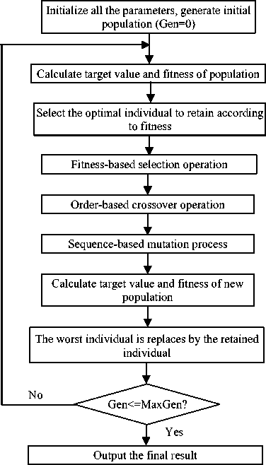
Figure 1. Genetic algorithm flow chart

5)    Calculation of the fitness

The processing time of each individual of population is a two-dimensional array which rows denote machines and columns denote work pieces. When we calculate the make span of scheduling which is the individual of population, we can use the code in Fig. 2. And the “Paixu” in the code denotes the processing time of a scheduling which is a specific arrangement of work pieces. Repeat the program with population size times, the target values of all individuals which are the make spans can be drawn. Due to the make span is better the value is few, it is opposite with the fitness. Therefore, in order to obtain the fitness the conversion formula is needed. There are two conversion formulas, one is the addition formula shown in formula 6, and the other is multiplication formula shown in formula 7.

FitnV j = max(ObjV) - ObjV j + 1 .     (6)

Where: j=1, 2,……, Npop

FitnVj denotes the fitness of individuals;

max(ObjV) denotes the largest processing time;

ObjVj denotes the processing time of j-individuals;

Through the transformation, the target value is smaller, the fitness value is greater, in order to avoid zero value of the fitness, the fitness value of every individual adds one.

FitnV j = max (ObjV) / ObjV j .      (7)

Where: j=1, 2,……, Npop

FitnVj denotes the fitness of individuals;

max(ObjV) denotes the largest processing time;

ObjVj denotes the processing time of j-individuals;

Because the individual target is Make span, its value is

[rows,cols]=size(paixu); sum(1)=paixu(1,1);

for i=1:rows-1

sum(i+1)=sum(i)+paixu(i+1);

end for i=2:rows for j=1:cols-1

sum(j*rows+1)=sum((j-

1)*rows+1)+paixu(j*rows+1);

sum(j*rows+i)=max(sum((j-1)*rows+i), sum(j*rows+i-1))+paixu(j*rows+i);

end end not zero, so the formula is available for all individuals.

Figure 2. The code of calculation of make span

6)    Select the retain optimal individual

Sort the population according to fitness, then the highest fitness as the best individual to retain. The detailed code is in Fig. 3.

[FitnV_bl, FitnI_bl]=sort(FitnV);

chrom N=chrom(FitnI bl(NIND) :);

Figure 3. The code of selection the retain individual

7)    Fitness-based selection operation

According to the fitness to generate a judgment which size is one row and Npop columns, and producing a random number which range is [0 1], if the comparison judgment, according to the location of judgment which is the random number would fall in to choose the corresponding individual, we can complete the selection operation by the code in Fig. 4.

[rows,cols,nums]=size(chrom_flowshop); chrow_flowsh=zeros(rows,cols,nums);

zhongjianshu=0;

pandanjz=zeros(1,NIND+1);

zongpandanshu=0;

for i=1:nums pandanjz1(i)=FitnV(i)+1-min(FitnV);

zongpandanshu=zongpandanshu+pandanjz1(i);

end for i=1:nums pandanjz2(i)=pandanjz1(i)/zongpandanshu;

pandanjz(i+1)=pandanjz(i)+pandanjz2(i);

end for i=1:nums

A=0;

xzs=rand(1,1);

for j=1:NIND if xzs>=pandanjz(j)&xzs<=pandanjz(j+1) A=j;

end if A>0 break; end end chrom_flowsh(:,:,i)=chrom_flowshop(:,:,A); end

Figure 4. The code of selection operation

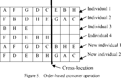
8)    Order-based crossover operation

On the basis of the select operation, choosing the first and second individuals, and randomly selecting the cross position, deleting the work pieces of 2nd individual which is the same as the work pieces of 1st individual before the cross position, and deleting the work pieces of 1st individual which is the same as the work pieces of 2nd individual after the cross position, with the rest of work pieces of 2nd individual to replace the work pieces of the 1st individual after the cross position, the new 1st individual is obtained, and with the rest of work pieces of 1st individual to replace the work pieces of the 2nd individual before the cross position, the new 2nd individual is obtained. The method is specifically described in Fig. 5.

9)    Order-based mutation operation

In order to ensure the feasibility of solutions, in the mutation operation, we can randomly select two locations; exchange the serial numbers of work pieces on the selected locations. So the mutation operation is completed and the new individual can meet the feasibility requirement. The specific code is in Fig. 6.

Calculating the individual fitness according to the target value of individuals in population is the second step of GA, the second program can be executed directly.

[rows,cols,nums]=size(chrom_gongxu);

jishu_weizhi=zeros(1,2);

pandanjz=zeros(1,1+cols);

for j=2:1+cols pandanjz(j)=pandanjz(j-1)+1/cols;

end for i=1:NIND while jishu_weizhi(1)==jishu_weizhi(2) jishu_weizhi=rand(1,2);

for j=1:2

jishu_weizhi(j)=k-1;

end if jishu_weizhi(j)==k-1 break end end end end x_pandan=rand(1,1);

if                     x_pandan

chrom_gongxu(:,jishu_weizhi(2),i)=zhongjianshu;

end end

Figure 6. The code of mutation operation

10) Replace the worst individuals with the best to generate a new population

After sort the individuals of population according to the fitness, and replace the first individual in the sequence with the best individual, the new population can be gained. The code is in Fig. 7.

[FitnV1,FitnI]=sort(FitnV);

chrom(:,:,FitnI(1))=chromN;

Figure 7. The code of replace operation

Finally, to determine whether the terminating condition is satisfied, if satisfied output the final result, if fail to satisfy go back to the second step repeated the GA until the terminating condition is satisfied.

• B.    Test of Car problems

We independently run the above two genetic algorithms 20 times to solve the Car kind problems from Car1 to Car8, and record the results of each run. The results show in Tab. 3, Tab. 4, Tab. 5 and Tab. 6.

Form the results we can see the GA whose initial population is improved by heuristic algorithm obtained more stable satisfactory solution and cost less genetic times, and without using the results of the heuristic algorithm, the solution quality is poor, and cost longer time. Since then, we can see that the proposed heuristic algorithm can effectively improve the result quality of intelligence algorithm.

TABLE III.        Comparisons of two GA on Car1 and Car2

run	Car1				Car1
	Sim GA		Imp GA		Sim GA		Imp GA
	Opt	gen	Opt	gen	Opt	gen	Opt	gen
1	7523	62	7038	1	8458	1	7166	1
2	7138	30	7038	1	8157	51	7166	1
3	7168	25	7038	1	7916	54	7166	1
4	7689	9	7038	1	7870	80	7166	1
5	7648	27	7038	1	7617	62	7166	1
6	7038	54	7038	1	7617	50	7166	1
7	7626	70	7038	1	8021	74	7166	1
8	7048	11	7038	1	7617	56	7166	1
9	7689	9	7038	1	7820	56	7166	1
10	7048	57	7038	1	8166	3	7166	1
11	7259	38	7038	1	7617	70	7166	1
12	7685	58	7038	1	8215	5	7166	1
13	7685	21	7038	1	8202	7	7166	1
14	7190	69	7038	1	8166	9	7166	1
15	7038	21	7038	1	7730	54	7166	1
16	7692	61	7038	1	8166	5	7166	1
17	7685	18	7038	1	7973	15	7166	1
18	7545	77	7038	1	7617	48	7166	1
19	7648	21	7038	1	8157	26	7166	1
20	7689	8	7038	1	8166	3	7166	1

Ave	7436.55	37.3	7038	1	7963.4	36.45	7166	1
Opt	7038	54	7038	1	7617	48	7166	1

TABLE IV.   Comparisons of two GA on Car3 and Car4

run	Car3				Car4
	Sim GA		Imp GA		Sim GA		Imp GA
	Opt	gen	Opt	gen	Opt	gen	Opt	gen
1	7710	15	7399	1	8479	38	8003	1
2	7531	57	7399	1	8714	74	8003	1
3	7919	62	7399	1	8564	78	8003	1
4	8171	45	7399	1	8426	54	8003	1
5	8126	18	7399	1	8423	61	8003	1
6	7543	62	7399	1	9487	1	8003	1
7	7594	5	7399	1	9487	2	8003	1
8	7770	27	7399	1	9487	33	8003	1
9	7543	51	7399	1	9487	5	8003	1
10	8590	5	7399	1	8611	64	8003	1
11	8567	24	7399	1	9487	7	8003	1
12	7981	50	7399	1	9487	4	8003	1
13	7800	59	7399	1	9487	3	8003	1
14	8255	80	7399	1	9487	2	8003	1
15	8682	8	7399	1	9487	3	8003	1
16	8380	16	7399	1	8423	73	8003	1
17	8099	67	7399	1	8611	23	8003	1
18	7954	80	7399	1	9487	5	8003	1
19	7741	76	7399	1	8917	58	8003	1
20	8126	22	7399	1	9487	1	8003	1
Ave	8004.1	41.45	7399	1	9076.25	29.45	8003	1
Opt	7531	57	7399	1	8423	61	8003	1

• TABLE V.    Comparisons of two GA on Car5 and Car6

  run	Car5				Car6
  	Sim GA		Imp GA		Sim GA		Imp GA
  	Opt	gen	Opt	gen	Opt	gen	Opt	gen
  1	8047	44	7720	42	9507	13	8570	73
  2	7843	79	7720	7	8754	11	8715	25
  3	8235	35	7808	1	9126	38	8739	1
  4	7862	45	7750	69	9355	55	8715	62
  5	7867	62	7720	24	8754	58	8715	36
  6	7845	17	7768	17	9170	16	8739	1
  7	7862	10	7750	16	9170	49	8739	1
  8	7825	8	7750	69	9404	10	8739	1
  9	7761	68	7720	12	9170	70	8715	47
  10	7865	9	7779	45	8852	60	8739	1
  11	8518	51	7750	30	9267	26	8715	3

  12	7835	58	7768	8	8813	37	8739	1
  13	8057	76	7808	1	8754	49	8570	3
  14	7822	62	7750	5	9293	6	8570	76
  15	7821	70	7720	13	9599	56	8570	13
  16	8003	10	7750	32	9187	14	8715	7
  17	7867	27	7808	1	8715	12	8715	40
  18	7865	6	7808	1	8742	59	8739	1
  19	8235	13	7750	59	9450	72	8739	1
  20	8039	11	7720	58	9179	33	8715	3
  Ave	7953.7	/	7755.85	/	9113.05	/	8695.6	/
  Opt	7761	68	7720	7	8715	12	8570	13

• TABLE VI.   Comparisons of two GA on Car7 and Car8

  run	Car7				Car8
  	Sim GA		Imp GA		Sim GA		Imp GA
  	Opt	gen	Opt	gen	Opt	gen	Opt	gen
  1	6685	48	6590	1	9014	15	8487	6
  2	6779	24	6590	1	9091	8	8530	1
  3	6887	19	6590	1	9265	59	8530	1
  4	6779	21	6590	1	8964	13	8479	3
  5	6803	77	6590	1	9313	49	8409	34
  6	6753	30	6590	1	9170	60	8530	1
  7	6887	13	6590	1	9170	41	8530	1
  8	7037	68	6590	1	9365	62	8530	1
  9	7084	54	6590	1	8505	71	8530	1
  10	6590	8	6590	1	9267	39	8479	2
  11	6753	12	6590	1	9504	5	8530	1
  12	6681	33	6590	1	9459	77	8366	22
  13	6753	16	6590	1	9068	20	8366	53
  14	6888	80	6590	1	9307	28	8530	1
  15	6983	7	6590	1	9170	49	8530	1
  16	6760	34	6590	1	8871	14	8530	1
  17	6753	10	6590	1	9170	22	8530	1
  18	6681	26	6590	1	9188	13	8530	1
  19	6753	38	6590	1	9226	15	8473	5
  20	6753	55	6590	1	8990	15	8530	1
  Ave	6802.1	33.65	6590	1	9153.85	33.75	8497.45	6.9
  Opt	6590	8	6590	1	8505	71	8366	22

V. Conclusion

Based on the number of work pieces, a new mixed constructive heuristic algorithm has been designed, and implemented through MATLAB. And contrasting with Dannenbring method, NEH method and Rajendran method by the problems of Car and Hel, the results prove that the new method is better than the other three methods, and it can effectively improve the make span. It can improve the Dannenbring result by 6.2%, and improve the NEH result 4%, and improve Rajendran result by 2.4%. And we discuss the application of the heuristic algorithm in GA. After designing two GAs, one is the simple GA, and the other is improved GA, we test the effect which the heuristic algorithm on GA by eight Car class problems. The result shows using the heuristic algorithm can improve the quality and speed of GA. It can improve the average value by 398.55 and average genetic times by 36.3 on Car. Although it can’t improve the optimal value on Car1, it can get the optimal solution with few times by 36.3. And the specific improvement on Car1-8 is in Tab.7 and Tab.8.

TABLE VII.   Improvement on values and genetic times on car1-4

	Car1		Car2		Car3		Car4
	Val	Gen	Val	Gen	Val	Gen	Val	Gen
Ave	398.55	36.3	797.4	35.45	605.1	40.45	1073.25	28.45
Opt	0	53	451	47	132	56	420	60

TABLE VIII. Improvement on values and genetic times on car5-8

	Car5		Car6		Car7		Car8
	Val	Gen	Val	Gen	Val	Gen	Val	Gen
Ave	197.85	12.55	417.45	17.4	212.1	32.65	656.4	26.85
Opt	41	61	145	-1	0	7	139	49

Acknowledgment

This paper was supported by National Natural Science Foundation of China under grant number 50875101 and Open Research Foundation of Green Manufacturing and Energy Conservation Technology Research Center under grant number C1010.