Design information technology of quantum algorithm gates

Author: Barchatova Irina, Degli Antonio Giovanni, Ulyanov Sergey
Journal: Сетевое научное издание «Системный анализ в науке и образовании» @journal-sanse
Article in issue: 3, 2014.
Free access
IT design of quantum algorithmic gates (QAG) is considered. General structures of the QAG design method and simulation system are introduced. Applications to efficient simulation of quantum algorithms (QA) on classical computer are described.
It design of quantum algorithmic gates, efficient simulation of quantum algorithms, general structure of the quantum algorithms
Short address: https://sciup.org/14122614
IDR: 14122614
Информационная технология проектирования квантовых алгоритмических ячеек
Рассмотрена информационная технология проектирования квантовых алгоритмических ячеек. Описываются общие структуры методов проектирования квантовых алгоритмических ячеек и их моделирования. Приведены приложения эффективного моделирования квантовых алгоритмов на классическом компьютере.
Text of the scientific article Design information technology of quantum algorithm gates
ИНФОРМАЦИОННАЯ ТЕХНОЛОГИЯ ПРОЕКТИРОВАНИЯ КВАНТОВЫХ АЛГОРИТМИЧЕСКИХ ЯЧЕЕК
Бархатова Ирина Александровна1, Джиованни дели Антонио2, Ульянов Сергей Викто-рович3
-
1Аспирант;
ГБОУ ВО «Международный Университет природы, общества и человека «Дубна»,
Институт системного анализа и управления;
141980, Московская обл., г. Дубна, ул. Университетская, 19;
-
2Доктор наук, профессор;
Поло дидаттико, Крема, факультет информационных технологий;
Италия, Крема, Виа Браманте, 65-26013;
-
3Доктор физико-математических наук, профессор;
ГБОУ ВО «Международный Университет природы, общества и человека «Дубна»,
Институт системного анализа и управления;
141980, Московская обл., г. Дубна, ул. Университетская, 19;
General structure of the quantum algorithmic gate (QAG) design method
Traditionally QA is written as a quantum circuit.
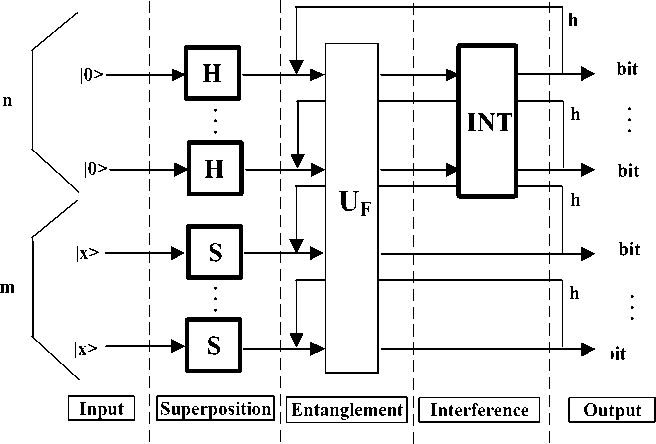
As shown in Fig. 1, the general structure of the quantum circuit is based on three quantum operators (superposition, entanglement, and interference) and measurement.
Repeated k times
M E A
U R E
E N
T
Figure 1. Quantum circuit structure
.
.
.
.
.
.
Input in the quantum circuit acts on an initial canonical basis vector to generate a complex linear combination (called a superposition) of basis vectors as an output. This superposition contains the information to answer the initial problem. After the superposition has been created, measurement takes place in order to extract the answer information. In quantum mechanics, a measurement is a non-deterministic operation that produces as output only one of the basis vectors in the entering superposition.
A general QA, written as a quantum circuit, can be automatically translated into the corresponding programmable quantum gate for efficient classical simulation. This gate is represented as a quantum operator in matrix form such that, when it is applied to the vector input representation of the quantum register state, the result is the vector representation of the desired register output state.
The simulation system of quantum computation is based on QAG’s.
The design process of QAG’s includes the matrix design form of three quantum operators: superposition (Sup) , entanglement ( U ) and interference (Int) that are the background of QA structures. In general form, the structure of a QAG can be described as follows (see Chapter 1):
QAG = [ ( Int ® n I ) • UF ] h + 1 •[ n H ® m S ] ,
where I is the identity operator; the symbol ® denotes the tensor product; S is equal to I or H and dependent on the problem description. One portion of the design process in Eq. (1) is the type-choice of the entanglement problem dependent operator U that physically describes the qualitative properties of the function f .
The efficient implementations of a number of operations for quantum computation include controlled phase adjustment of the amplitudes in the superposition, permutation, approximation of transformations and 2
generalizations of the phase adjustments to block matrix transformations. These operations generalize those used as example in quantum search algorithms (QSA’s) that can be realized on a classical computer. The application of this approach is applied herein to the efficient simulation on classical computers of the Deutsch QA, the Deutsch–Jozsa QA, the Simon QA, the Shor QA and the Grover QA.
Implementation of a QA is based on a QAG. In the language of classical computing, a quantum computer is programmed by designing a QAG. The prior art reports relatively few such gates because the basic principles underlying the quantum version of programming are in their infancy and algorithms to date have been programmed by ad-hoc techniques.
Fig. 2 is a block diagram showing a gate approach for simulation of a QA using classical computers.
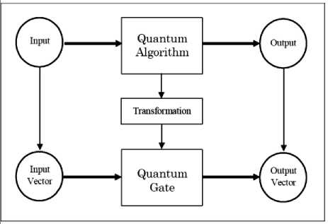
Figure 2. The gate approach for simulation of quantum algorithms using classical computers
In Fig. 2, an input is provided to a QA and the QA produces an output. However, the QA can be transformed to produce a QAG such that an input vector (corresponding to the QA input) is provided to the QAG to produce an output vector (corresponding to the QA output).
Fig. 3 is a block diagram showing the design of the QAG.
In Fig. 3, an input block of the QA is a function f that maps binary strings into binary strings. This function f is represented as a map table block, defined for every string its image. The function is first encoded in corresponding block into a unitary matrix operator U depending on the properties of f . In some sense, this operator calculates f when its input and output strings are encoded into canonical basis vectors of a complex Hilbert space.
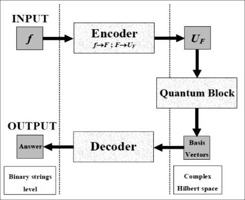
Figure 3. Schematic block diagram of QAG method design
The operator U maps the vector code of every string into the vector code of its image by f . The quantum block operates on basis vectors in a complex Hilbert space. The vectors operated on by the quantum 3
Электронный журнал «Системный анализ в науке и образовании» Выпуск №3, 2014 год block are provided to a decoder, which decodes the vectors to produce an answer. Once generated, the matrix operator U F is embedded into a quantum gate G .
The quantum gate G is a unitary matrix whose structure depends on the form of matrix U F and on the problem to be solved. The quantum gate is a unitary operator built from the dot composition of other more specific operators. The specific operators are described as tensor products of smaller matrices.
The quantum circuit is a high-level description of how these smaller matrices are composed using tensor and dot products in order to generate the final quantum gate as shown in Fig. 1.The mathematical background of this approach is based on mappings between the quantum block operations in the complex Hilbert space. The encoder and decoder operate in a map table and interpretation space, and input/output occurs on a binary string level. The Clifford and Pauli groups are the background for universal QAG design for simulation of a QA’s on classical computers.
The probability of every basis vector of being the output of measurement depends on its complex coefficient (probability amplitude) in the entering complex linear combination.
Main QAG’s and main quantum operators
Three quantum operators, superposition, entanglement, and interference, are the basis for quantum computations of qualitative and quantitative measures in quantum soft computing. As described above, Fig. 3 shows the structure of a QAG based on the three quantum operations of superposition, entanglement, and interference.
Fig. 4 shows methods in QAG design.
The methods as shown in Fig. 4 are based on qualitative measures of QAG design: 1) analysis of QA dynamics and structure gate design; 2) analysis of information flow; and 3) structure simulation of intelligent QA’s on classical computers.
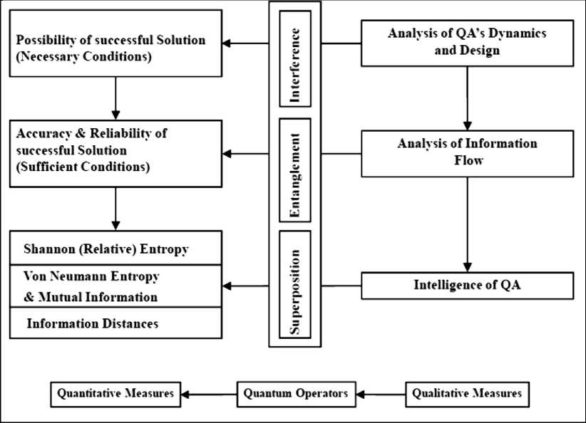
Figure 4. Methods in Quantum Algorithm Gate Design
In this paper analysis of QA dynamics and structure gate design, and structure simulation of intelligent QA’s on classical computers are discussed.
As shown in Fig. 4 analysis of QA dynamics provides the background for showing the existence of a solution and that the solution is unique with the desired probability. Analysis of information flow in the QA 4
gates provides the background for showing that the unique solution exists with the desired accuracy and that the reliability of the solution can be achieved with higher probability.
With the method of quantum gate design presented herein, various different structures of QA can be realized, as shown in Table 1 below.
The intelligence of a QA is achieved through the principle of minimum information distance between Shannon and von Neumann entropy and includes the solution of the QA stopping problem.
The output states of a QA as the solution of expected problems are the intelligent states with minimum entropic relations of uncertainty (coherent superposition states). The successful results of QA computing are robust to noise excitations in quantum gates, and intelligent quantum operations are fault-tolerant in quantum soft computing.
Table 1. Quantum gate parameters for QA’s structure design
|
Name |
Algorithm |
Gate Symbolic F Г ""I h +1 ( Int ® mI ) • UF • Entanglement L Interference _ |
orm: ( ^ nH ® mS X__________ __________/ у Superposition у |
|
Deutsch-Jozsa (D. – J.) |
m = 1, S = H ( x = 1) Int = nH k = 1 h = 0 |
( nH ® I ) • u D . - J . • ( |
n + 1 H ) |
|
Simon (Sim) |
m = n, S = I ( x = 0) Int = nH k = O ( n ) h = 0 |
( nH ® nI ) • U Sm • ( nH ® nI ) |
|
|
Shor (Shr) |
m = n, S = I ( x = 0) Int = QFT n k = O ( Poly ( n ) ) h = 0 |
( QFTn ® nI ) • Up' ' • ( nH ® nI ) |
|
|
Grover (Gr) |
m = 1, S = H ( x = 1) Int = D„ k = 1, h = O ( 2 n /2 ) |
( D n ® I ) • U G • ( n + 1 H ) |
|
A quantum computer is difficult to build because of decoherence effects.
Decoherence introduces errors in the superposition.
The decoherence problem is reduced by using tools of quantum soft computing such as a quantum genetic search algorithm (QGSA). Errors produced by decoherence are of three kinds: (i) phase errors; (ii) bitflip errors; and (iii) both phase and bit-flip errors. These three errors can all be modeled using unitary transformations.
This means that if the QGSA is implemented on a physical quantum-mechanical system, one would gain the advantages of quantum parallelism and reduce the problem of decoherence, because decoherence can be used as a natural generator of mutation and crossover operators.
Design technology of quantum algorithmic gate boxes and simulation system
The problems solved by the QA can be stated as follows:
|
Input |
A function f : {0,1} n ^ {0,1} m |
|
Problem |
Find a certain property of f |
The structure of a quantum operator U in QA’s as shown in block of Fig. 3 is outlined, with a high level representation, in the scheme diagram Fig. 1. In Fig. 3 the input of the QA is a function f that maps from binary strings into binary strings. This function is represented as a map table, defining for every string its image. The function f is encoded according to an F -truth table. The function is transformed according to a transform U -truth table into a unitary matrix operator U F depending on f’ s properties. In some sense, this operator calculates f when its input and output strings are encoded into canonical basis vectors of a complex Hilbert space: U F maps the vector code of every string into the vector code of its image by f . A squared matrix U F on the complex field is unitary if and only if (iff) its inverse matrix coincides with its conjugate transpose: U - 1 = U . A unitary matrix is always reversible and preserves the norm of vectors.
Fig. 5 shows structure of the quantum block from Fig. 3.
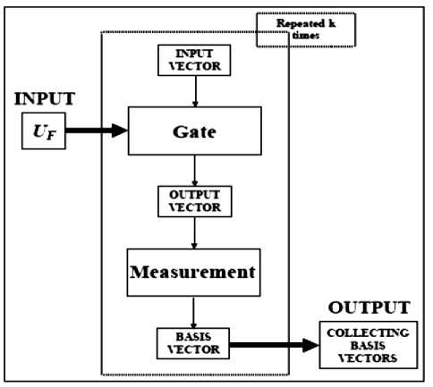
Figure 5. Structure of Quantum Block in Fig. 3
In the structure, the matrix operator U F has been generated it is embedded into a quantum gate as a QAG, a unitary matrix whose structure depends on the form of matrix U F and on the problem to be solved. In the QA, the QG acts on an initial canonical basis vector (which can always choose the same vector) in order to generate a complex linear combination (superposition) of basis vectors as output. This superposition contains all the information to answer the initial problem.
After this superposition has been created, in measurement block takes place in order to extract this information. In quantum mechanics, measurement is a non-deterministic operation that produces as output only one of the basis vectors in the entering superposition. The probability of every basis vector of being the output of measurement depends on its complex coefficient (probability amplitude) in the entering complex linear combination.
The segmental action of the QAG and of measurement characterizes the quantum block in Fig. 5. The quantum block is repeated k times in order to produce a collection of k basis vectors. Since measurement a nondeterministic operation, these basic vectors are not be necessarily identical and each one of them will encode a piece of the information needed to solve the problem. The collection block in Fig. 3.5 of the algorithm outputs the interpretation of the collected basis vectors in order to get the answer for the initial problem with a certain probability.
Encoder
The behavior of the encoder in Fig . 3 is described in the scheme diagram of Fig. 6. Function f is encoded into matrix U F in three steps.
In step 1, the map table ( f - truth table ) of function f : {0,1} n → {0,1} m is transformed into the map table ( F - truth table) of the injective function F :{0,1} n+m → {0,1} n+m such that:
F ( X 0 , .., X n -1 , y 0 , .., y m -1 ) = ( X 0 , .., X n-1 , f(X 0 , .., X n -1 ) ® ( y 0 , .., y m -1 )).
Remark . The need to deal with an injective function comes from the requirement that U F is unitary. A unitary operator is reversible, so it cannot map 2 different inputs in the same output. Since U F will be the matrix representation of F , F is injective. If one directly employed the matrix representation of function f , one could obtain a non-unitary matrix, since f could be non-injective. So, injectivity is fulfilled by increasing the number of bits and considering function F instead of function f . The function f can be calculated from F by putting ( y 0 ,..., y m -1 ) = (0,...,0) in the input string and reading the last m values of the output string.
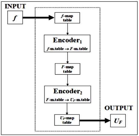
Figure 6. The encoder block scheme diagram
Reversible circuits realize permutation operations. It is possible to realize any Boolean circuit F : В n ^ B m by reversible circuit. For this case, one need not calculate the function F : В n ^ B m . One can calculate another function with expanding F^ :B n + m ^ B n + m that is defined as following relation: F^ ( x , y ) = ( x, y ® F ( x ) ) where the operation ® is defined as addition on module 2.
Then the value of F ( x ) is defined as F^ ( x ,0 ) = ( x, F ( x ) ) . For example, the XOR operator between two binary strings p and q of length m is a string s of length m such that the i -th digit of s is calculated as the exclusive OR between the i -th digits of p and q :
p = (p o , .., p n -1 ), q = ( q o , .., q n -1 ); 5 = p ® q = ((p 0 + q 0 ) mod 2, .., (p n -1 + q n -1 ) mod 2)).
In step 2, the function from F map table is transformed into U F map table, according to the following constraint:
-
V 5 e {0,1} n + m : U f [ t (s )] = t [ F ( 5 )] (2)
The code map T : {0,1} n + m ^ C2 n + m (C2 n + m is the target Complex Hilbert Space) is such that:
T (0 ) = LI = | 0), T (1)=,! = b)
-
V 0 ) V 1 ) .
T ( xtiV, xn + m - 1 ) = T ( x 0 ) ® ■ ■ ■ ® T ( x n + m - 1 ) = I x 0 ■ " " x n + m - 1)
Code T maps bit values into complex vectors of dimension 2 belonging to the canonical basis of C 2. Besides, using tensor product, T maps the general state of a binary string of dimension n into a vector of dimension 2 n , reducing this state to the joint state of the n bits composing the register. Every bit state is transformed into the corresponding 2-dimesional basis vector and then the string state is mapped into the corresponding 2 n -dimesional basis vector by composing all bit-vectors through tensor product. In this sense tensor product is the vector counterpart of state conjunction.
The tensor product between two vectors of dimensions h and k is a tensor product of dimension h • k , such that:
( x i У 1 1
x 1 U y 1
x 1 yk
...
xh y 1
... ® ...
V xh 7 V yk 7
V x h y k 7
If a component of a complex vector is interpreted as the probability amplitude of a system of being in a given state (indexed by the component number), the tensor product between two vectors describes the joint probability amplitude of two systems of being in a joint state.
For example:
f 0 1
(0,0)

100), (0,1)


101\
(1,0)
f 0 1 0

(1,1)

f 0 1 0
IH).
Basis vectors are denoted using the ket notation i . This notation is taken from Dirac description of quantum mechanics.
In step 3, the U F map table is transformed into U F using the following transformation rule:
[Uf] i= 1 о Uf^ = |i).
This rule can be understood by considering vectors i and j as column vectors. These vectors belong to the canonical basis, where U F defines a permutation map of the identity matrix rows. In general, row j is mapped into row i .
This rule will be illustrated in detail below, in the example based on Deutsch’s algorithm.
Quantum block
The heart of the quantum block is the quantum gate, which depends on the properties of matrix U F . The quantum block uses the QAG, which depends on the properties of matrix U F . The structure of a quantum operator U in QA’s as shown in Fig. 3 is outlined, with a high level representation, in the scheme diagram of Fig. 5.
The scheme in Fig. 5 gives a more detailed description of the quantum block. The matrix operator U F of Fig. 6 is the output of the encoder block represented in Fig. 3.
Here, it becomes the input for the quantum block. This matrix operator is embedded into a more complex gate: the gate G (QAG). Unitary matrix G is applied k times to an initial canonical basis vector i of dimension 2n+m. Each time, the resulting complex superposition G 0 01 1 of basis vectors is measured in measurement block, producing one basis vector |xj as result. The measured basis vectors {x,...,xk} are collected together in block of basis vectors.
This collection is the output of the quantum block. The “intelligence” of the QA’s is in the ability to build a QAG that is able to extract the information necessary to find the required property of f and to store it into the output vector collection.
In order to represent QAGs it is useful to employ some diagrams called quantum circuits, as shown in Fig. 1. Each rectangle is associated with a matrix 2 n x 2 n , where n is the number of lines entering and leaving the rectangle. For example, the rectangle marked U F is associated with the matrix U F .
Using a high-level description of the gate and, using transformation rules shown in Fig. 7, it is possible to compile the corresponding gate-matrix.
These rules are listed in Fig. 7 as following: (a) Rule 1 – Tensor Product Transformation; (b) Rule 2 – Dot Product Transformation; (c) Rule 3 – Identity Transformation; (d) Rule 4 – Propagation Rule; (e) Rule 5 – Iteration Rule; and (f) Rule 6 – Input/Output Tensor Rule.
It will be clearer how to use these rules when we afford the first examples of quantum algorithm.
The tensor product between two matrices X nxm and Y hxk is a (block) matrix ( n • h ) x ( m • k ) such that:
x 11 Y .. x 1 mY
x 11
X ® Y =
with X =
xn 1 Y .. xnmY
xn 1
x1m xnm
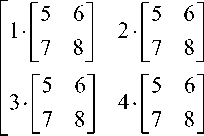
An example of a matrix tensor product is as follows:
2 1 Г 5
®
4 7
|
5 |
6 |
10 |
12 |
|
7 |
8 |
14 |
16 |
|
15 |
18 |
20 |
24 |
|
21 |
24 |
28 |
32 |
Decoder
The decoder block of Fig. 3 interprets the basis vectors (collected in block basis vectors) of after the iterated execution in the quantum block. Decoding these vectors involves retranslating them into binary strings and interpreting them directly in decoder block if they already contain the answer or use them, for instance as coefficients vectors for some equation system, in order to get the searched solution.
Examples of design method application: QA’s Benchmark’s gate design and simulation of decision making QA
Let us consider Benchmarks of QAG design for typical QA.
Deutsch’s algorithm
In order to illustrate the general method to synthesize a QA and the QG implementing it, a simple pedagogical example, Deutsch’s algorithm, is used. The roles of superposition, entanglement and parallel quantum massive calculation are illustrated by this example.
Deutsch’s problem : A function f: {0,1} ^ {0,1} is said constant iff 3 y e {0,1}: V x e {0,1}: fx )= y . It is said to be balanced iff |{ x e {0,1}: fx )=0}| = |{ x e {0,1}: fx )=1}|.
Thus, Deutsch’s problem can be stated as follows:
|
Input |
A balanced or constant function f |
|
Problem |
Decide if f is constant or balanced |
Figure 8 shows the structure of Deutsch’s problem.
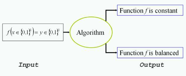
Figure 8. Problem definition of Deutsch’s QA
There are four possible functions f : {0,1} ^ {0,1}.
They are defined by the following map tables:
|
Constant Functions |
Balanced Functions |
|
(1) |
x |
f - ( x ) |
(3) |
x |
f К x ) |
||||
|
0 |
0 |
0 |
0 |
||||||
|
1 |
0 |
1 |
1 |
||||||
|
(2) |
x |
f = ( x ) |
(4) |
x |
f • ( x ) |
||||
|
0 |
1 |
0 |
1 |
||||||
|
1 |
1 |
1 |
0 |
||||||
The set { f i } i ∈ {1,2,3,4} is the input set for our algorithm.
Every function f i is represented by its map table.
Fig. 9 shows definitions of constant and balanced functions.
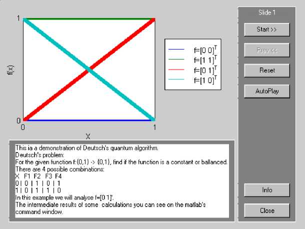
Figure 9. Deutsch’s quantum algorithm simulation: Problem definition visualization
Encoder . The encoder block encodes input function f into matrix U F . If, for example, the function to be investigated is f = f 3 , then the map table is the following:
|
x |
f К x ) |
|
0 |
0 |
|
1 |
1 |
Step 1
Function f is first transformed into function F :{0,1}2 → {0,1}2 such that
In logic representation this means:
F ( x 0 , y 0 ) = ( x 0 , f ( x 0 ) ⊕ y 0 ).
|
J 0 |
F ( x 0 , J o ) |
|
0 |
( x 0 , f ( x 0 )) |
|
1 |
( x 0 , f ( x 0 )) |
As usual, the NOT operator acting on a binary string flips the value of every digit in the string p = (p0, ..., pn-1), p = ((p0+1)mod2, ..., (pn-1+1)mod2).
Therefore, if f = f 3 , F- map table is the following:
|
( x 0 , y 0 ) |
F ( x 0 , y 0 ) |
|
(0,0) |
(0,0) |
|
(0,1) |
(0,1) |
|
(1,0) |
(1,1) |
|
(1,1) |
(1,0) |
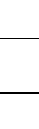
Fig. 10 shows the result of F -map table building.
Step 2
In this step, the map table of F is transformed into the map table of U F .
The transformation rule is the following:
∀ s ∈ {0,1}2: U F [ τ ( s )]= τ [ F ( s )].
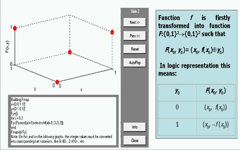
Figure 10. Deutsch’s quantum algorithm simulation, Step 1: F-map table building
So, U F map table is:
|
1 x 0 y 0 ) |
U F 1 x 0 y 0 ) |
|
1 00 |
1 00 ) |
|
1 01 |
1 01 ) |
|
1 10 |
111 |
|
111 |
1 10) |
|
v |
UF v |
|
(1,0,0,0) T |
(1,0,0,0) T |
|
(0,1,0,0) T |
(0,1,0,0) T |
|
(0,0,1,0) T |
(0,0,0,1) T |
|
(0,0,0,1) T |
(0,0,1,0) T |
The TRANSPOSE ( T ) operator acting on a row or column vector transforms the vector into its corresponding column or, row vector (respectively):
Г Х1 )
Г x 1
T
( X
xn ) T =
= ( x 1
xn ) .
v xn; v xn;
Step 3
The matrix associated with such a map table is obtained from the identity matrix 4 x 4 by a permutation of its rows: the first and the second rows are mapped into themselves, whereas the third row is mapped into the fourth one and the fourth row into the third one:
|
"1 0 0 0" 0 10 0 |
|
|
UF = |
0 0 0 1 , 0 0 10 , |
A general way to build U F is to express every vector U F ( s ) as a linear combination of the basis vectors. The coordinates of this combination are all 0, unless for one basis vector corresponding to the image of s by U F :
UF |00) = 1|00> + 0|01> + 0|10> + 0|11)
UF |01> = 0|00> + 1|01> + 0|10> + 0|11> UF |10> = 0|00> + 0|01> + 0|10> + 1|11>.
UF |11) = 0|00> + 0|01) + 1|10> + 0|11)
Calculate [ U F ] ij as the coordinate of vector U F ( j ) with respect to vector i , where i and j are binary sequences. This means:
[Ur 1, =1» UfI, = I').
Value [ U F ] ij is called the probability amplitude of j being mapped i into by U F .
The probability amplitude of 00 of being mapped into 00 is, for instance, 1, since U F 00 =1 00 , whereas its probability amplitude of being mapped into 01 is 0, since U F 00 =0 01 . Using this technique, the following unitary matrix is built:
|
U F |
00 |
01 |
|10 |
11 |
|
00 |
1 |
0 |
0 |
0 |
|
01 |
0 |
1 |
0 |
0 |
|
1 10) |
0 0 0 1 |
|
111н |
0 0 1 0 |
Fig. 11 shows the design process of unitary matrix U F .
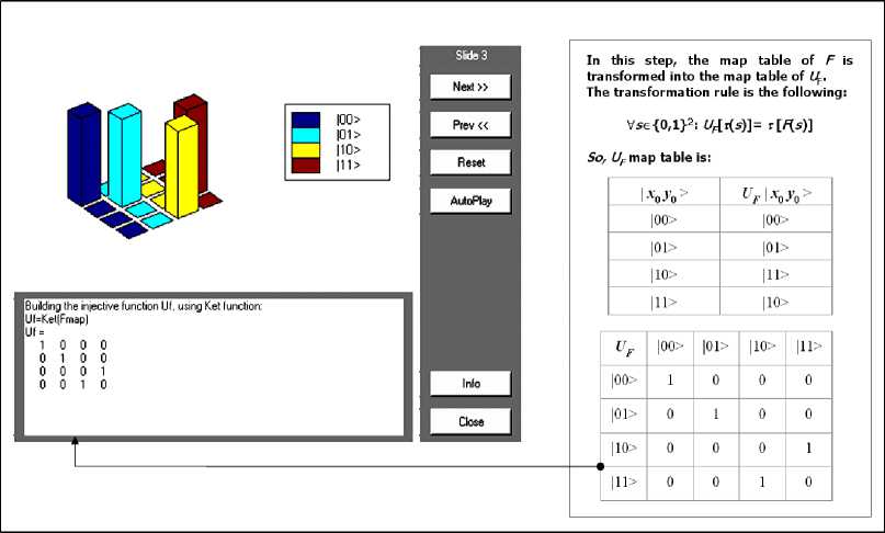
Figure 11. Deutsch’s quantum algorithm simulation, Step 2: Entanglement operator
Quantum block. The encoder block has generated matrix U F . This matrix is now embedded into the QG that will act on the input vector 00 .
Fig. 12 (a) shows this gate using a quantum circuit.
Figure 12. Deutsch’s quantum algorithm simulation:
Circuit representation and corresponding gate design
Each rectangle in Fig. 12 (a) represents a classical matrix operator n x n , where n is the number of lines entering and leaving the rectangle.
A matrix operator is said classical, when it maps every basis vector into another basis vector. For example, operator U F is classical. A thick rectangle stands for a non-classical matrix operator. A non-classical matrix operator maps at least one basis vector into a superposition of basis vectors.
Example : Classical and Non-Classical Matrix operators.
Classical Matrix Operator U F Non-Classical Matrix Operator H
|
U F |
00 |
01 |
10 |
11 |
||||
|
00 |
1 |
0 |
0 |
0 |
H |
0 |
1 |
|
|
01 |
0 |
1 |
0 |
0 |
0 |
1 21/2 |
1 21/2 |
|
|
10 |
0 |
0 |
0 |
1 |
1 |
1 21/2 |
- 1/2 1/2 |
|
|
11 |
0 |
0 |
1 |
0 |
||||
The above circuit is compiled into the corresponding computable gate. The first passage involves completing the circuit making some operators explicit. Consider, for instance, Step 1 in Fig. 12 (a). The second line is empty in this step. This means that the second entering basis vector is left unchanged. This vector acts in the identity matrix operator and completes the circuit. This is rule 3 described in Fig. 7. The result of the compilation is presented on the Fig. 12 (b). T he identity matrix o perator is classical and it is so defined as:
I 01
0 10
-
1 01
At this point a matrix operator is built corresponding to every step whose action corresponds to the concurrent action of the matrix operators acting on parallel lines. Rules 1 and 6 from Fig. 7 are used to obtain as the quantum circuit of Fig. 12 (c).
Finally, unique matrix operator is built that is equivalent to the sequential application of the operators in step 1, step 2 and step 3. This is operator composition and it is obtained with the dot product among matrices in the r everse order of application, as rule 2 states. Applying rule 2 from the Fig. 7 to the circuit yields as the quantum circuit of Fig. 12 (d), namely the programmable gate implementing Deutsch’s algorithm.
Figure 13 shows the result of computer design of QG of Deutsch's QA.
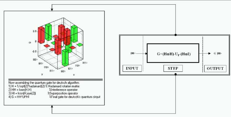
Figure 13. Deutsch’s quantum algorithm simulation, Step 4: Quantum gate assembling
Computational steps of design process. To compute and design the gate, first calculate ( H ® I) . The output matrix is 4 x 4. Label each column and row with the corresponding basis vector. Calculate the amplitude probability for each basis vector of being mapped into another basis vector using H and I . Take vector |00> for instance: its probability amplitude of being transformed into |01> is the product between the probability amplitude of |0> of being mapped into |0> by H and the probability amplitude of |0> of being transformed into |1> by I . This is the tensor product.
Therefore:
|
I |
|0> |
|1> |
|
|0> |
1 |
0 |
|
|1> |
0 |
1 |
The values H ® I and H ^ H are calculated as follows:
|
H ® I |
|00> |
|01> |
|10> |
|11> |
|
|00> |
1/21/2 |
0 |
1/21/2 |
0 |
|
|01> |
0 |
1/21/2 |
0 |
1/21/2 |
|
|10> |
1/21/2 |
0 |
-1/21/2 |
0 |
|
|11> |
0 |
1/21/2 |
0 |
-1/21/2 |
|
H ® H |
|00> |
|01> |
|10> |
|11> |
|
|00> |
1/2 |
1/2 |
1/2 |
1/2 |
|
|01> |
1/2 |
-1/2 |
1/2 |
-1/2 |
|
|10> |
1/2 |
1/2 |
-1/2 |
-1/2 |
|
|11> |
1/2 |
-1/2 |
-1/2 |
1/2 |
One can rewrite U F when f = f 3 :
|
U F3 |
|00> |
|01> |
|10> |
|11> |
|
|00> |
1 |
0 |
0 |
0 |
|
|01> |
0 |
1 |
0 |
0 |
|
|10> |
0 |
0 |
0 |
1 |
|
|11> |
0 |
0 |
1 |
0 |
The final programmable gate G 3 = ( H ® H) • ( Uf3 • ( H ® I)) is obtained as:
|
U F ⋅ ( H ⊗ I ) |
|00> |
|01> |
|10> |
|11> |
|
|00> |
1/21/2 |
0 |
1/21/2 |
0 |
|
|01> |
0 |
1/21/2 |
0 |
1/21/2 |
|
|10> |
0 |
1/21/2 |
0 |
-1/21/2 |
|
|11> |
1/21/2 |
0 |
-1/21/2 |
0 |
|
G 3 |
|00> |
|01> |
|10> |
|11> |
|
|00> |
1/21/2 |
1/21/2 |
0 |
0 |
|
|01> |
0 |
0 |
1/21/2 |
-1/21/2 |
|
|10> |
0 |
0 |
1/21/2 |
1/21/2 |
|
|11> |
1/21/2 |
-1/21/2 |
0 |
0 |
To calculate the programmable gates for the other possible input functions, the map tables are as follows:
|
x |
f - ( x ) |
|
0 |
0 |
|
1 |
0 |
|
( x 0 , J 0 ) |
F i ( x о , J 0 ) |
|
(0,0) |
(0,0) |
|
(0,1) |
(0,1) |
|
(1,0) |
(1,0) |
|
(1,1) |
(1,1) |
|
x |
f 2 ( X ) |
|
0 |
1 |
|
1 |
1 |
|
( X 0 , J о ) |
F 2 ( X 0 , J 0 ) |
|
(0,0) |
(0,1) |
|
(0,1) |
(0,0) |
|
(1,0) |
(1,1) |
|
(1,1) |
(1,0) |
From every table, it is easy to calculate the matrix operator:
|
| X 0 J 0 > |
U r1 | x 0 J 0 > |
|
|00> |
|00> |
|
|01> |
|01> |
|
|10> |
|10> |
|
|11> |
|11> |
|
UF1 |
|00> |
|01> |
|10> |
|11> |
|
|00> |
1 |
0 |
0 |
0 |
|
|01> |
0 |
1 |
0 |
0 |
|
|10> |
0 |
0 |
1 |
0 |
|
|11> |
0 |
0 |
0 |
1 |
|
| X 0 J 0 > |
U f2 | X о J o > |
|
|00> |
|01> |
|
|01> |
|00> |
|
|10> |
|11> |
|
|11> |
|10> |
|
UF2 |
|00> |
|01> |
|10> |
|11> |
|
|00> |
0 |
1 |
0 |
0 |
|
|01> |
1 |
0 |
0 |
0 |
|
|10> |
0 |
0 |
0 |
1 |
|
|11> |
0 |
0 |
1 |
0 |
|
( X 0 , J o ) |
U f4 | X о J o > |
|
|00> |
|01> |
|
|01> |
|00> |
|
|10> |
|10> |
|
|11> |
|11> |
|
UF4 |
|00> |
|01> |
|10> |
|11> |
|
|00> |
0 |
1 |
0 |
0 |
|
|01> |
1 |
0 |
0 |
0 |
|
|10> |
0 |
0 |
1 |
0 |
|
|11> |
0 |
0 |
0 |
1 |
Different U F ( i =1,2,4) generate different programmable gates G i =( H ⊗ H ) ⋅ U F ⋅ ( H ⊗ I ):
|
G 1 |
|00> |
|01> |
|10> |
|11> |
|
|00> |
1/21/2 |
1/21/2 |
0 |
0 |
|
|01> |
1/21/2 |
-1/21/2 |
0 |
0 |
|
|10> |
0 |
0 |
1/21/2 |
1/21/2 |
|
|11> |
0 |
0 |
1/21/2 |
-1/21/2 |
|
G 2 |
|00> |
|01> |
|10> |
|11> |
|
|00> |
1/21/2 |
1/21/2 |
0 |
0 |
|
|01> |
-1/21/2 |
1/21/2 |
0 |
0 |
|
|10> |
0 |
0 |
1/21/2 |
1/21/2 |
|
|11> |
0 |
0 |
-1/21/2 |
1/21/2 |
|
G 4 |
|00> |
|01> |
|10> |
|11> |
|
|00> |
1/21/2 |
1/21/2 |
0 |
0 |
|
|01> |
0 |
0 |
-1/21/2 |
1/21/2 |
|
|10> |
0 |
0 |
1/21/2 |
1/21/2 |
|
|11> |
-1/21/2 |
1/21/2 |
0 |
0 |
Finally, different programmable gates generate different superposition states:
|
G 1 |00> |
= |
1/21/2 |
|00> |
+ |
1/21/2 |
|01> |
|
G 2 |00> |
= |
1/21/2 |
|00> |
- |
1/21/2 |
|01> |
|
G 3 |00> |
= |
1/21/2 |
|00> |
+ |
1/21/2 |
|11> |
|
G 4 |00> |
= |
1/21/2 |
|00> |
- |
1/21/2 |
|11> |
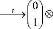
Observe that G 1 |00> and G 2 |00> can be written as the tensor products of two simpler vectors:
|
G 1 |00> |
= |
1/21/2 |0> ⊗ ( |0> + |1> ) |
|
G 2 |00> |
= |
1/21/2 |0> ⊗ ( |0> - |1> ) |
This is not possible for G 3 |00> and G 4 |00>. These two vectors make two entangled states.
This means that Deutsch’s QA needs entanglement for speed-up of quantum parallel massive calculations.
A vector v of dimension 2n is said to represent an entangled state if and only if it cannot be written as the tensor product of n vectors of dimension 2. Mathematically, the entanglement condition is written as:
-
-3 v i ,..., V n : v = V j ® ... ® V n
Figs 14 and 11 show the result of computer check of entanglement property.
When the QAG has generated the output vector, which is a linear complex superposition of basis vectors measurement takes place. It is assumed that measurement is a non-deterministic operation whose input is the linear superposition of basis vectors and whose output is only one of these basis vectors. The probability of a basis vector being the result of measurement is given by the squared modulus of its complex coordinate in the starting superposition.
This description of measurement is taken from quantum mechanics and it is the main constraint on the access one has to the results of the QAG. The non-deterministic evolution of a quantum system by measurement is the true qualitative difference between a quantum computation and a simple parallel computation.
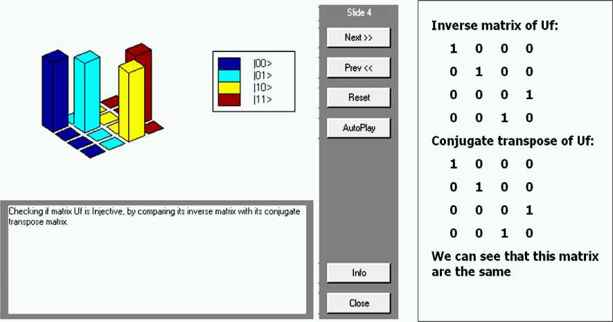
Figure 14. Deutsch’s quantum algorithm simulation, Step 3: checking if entanglement operator is injective or not
In quantum mechanics measurement is a non-deterministic operator. Writing a vector v as the complex linear combination of n basis vector v , * = 1’’”’ n the probability to observe v when v is measured is given by the squared modulus of the complex co-ordinate of v i in v .
У = а х у 1 + a у 2 + ... + а пу „
Measurement
|
Vector |
Probability |
||
|
v 1 |
а 1 |
2 |
|
|
v 2 |
« 2 |
2 |
|
|
v n |
a n |
2 |
|
When applying measurement to the superposition of basis vectors resulting from one of our 4 gates, the following is obtained:
|
Superposition of basis vectors ( before a measurement ) |
Result of measurement |
|
|
Vector |
Probability |
|
|
G i |00>=1/ ^ 2 |00> + 1/ ^ 2 |01> |
|00> |01> |
||1/ ^ 2||2=0.5 ||1/ ^ 2||2=0.5 |
|
G 2 |00>=1/ ^ 2 |00> - 1/ ^ 2 |01> |
|00> |01> |
||1/ ^ 2||2=0.5 ||1/ ^ 2||2=0.5 |
|
G з |00>=1/ ^ 2 |00> + 1/ ^ 2 |11> |
|00> |11> |
||1/ ^ 2||2=0.5 ||1/ ^ 2||2=0.5 |
|
G 4 |00>=1/ ^ 2 |00> - 1/ ^ 2 |11> |
|00> |11> |
||1/ ^ 2||2=0.5 ||1/ ^ 2||2=0.5 |
With measurement, the quantum block ends. In Deutsch’s algorithm the quantum block is repeated only one time, so only one resulting basis vector is collected. Thus for success result of decision making is enough 50% of probability.
Decoder. When the final basis vector has been produced, it is interpreted to find the information it carries in order to establish if f is constant or balanced. If the resulting vector is |00> nothing can be said about which function was encoded in U F . But if the result is |01> or |11>, the function was f 1 or f 2 in the first case, f 3 or f 4 in the second. In fact only gates G 1 and G 2 may produce a vector such that, when it is measured, basis vector |01> has a non-null probability of being observed. Similarly, only gates G 3 and G 4 may produce a superposition of basis vectors where vector |11> has non-null probability amplitude. Since f 1 and f 2 are constant, whereas f 3 and f 4 are balanced, the resulting vector is easily decoded in order to answer Deutsch’s problem:
|
Resulting vector ( after measurement ) |
Answer |
|
|00> |
Nothing can be said |
|
|01> |
f is constant |
|
|11> |
f is balanced |
The above described design and calculation processes of QAG for Deutsch’s QA can be efficiently simulated on computers with Von Neumann architecture.
Computer design process of Deutsch’s QAG and simulation results. Fig. 15 shows the result of computer design of superposition and interference quantum operators.
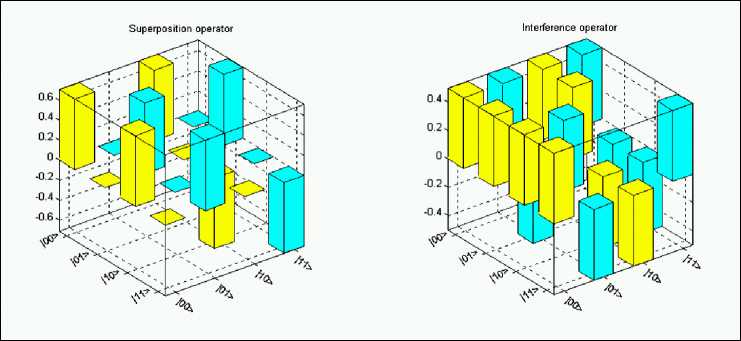
Figure 15. Deutsch’s quantum algorithm: Superposition and Interference operators
Fig. 16 shows the result of QG assembly and results of numerical data simulation using this QAG.
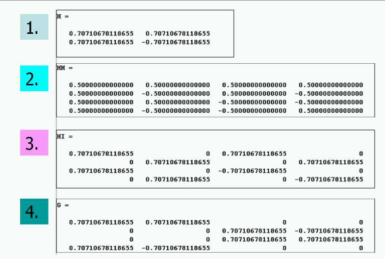
Figure 16. Deutsch’s quantum algorithm simulation, Step 4: Quantum gate assembling, results of calculations
Fig. 17 shows the general results of decision-making Deutsch’s QA for fourth different cases.
Constant functions Balanced functions
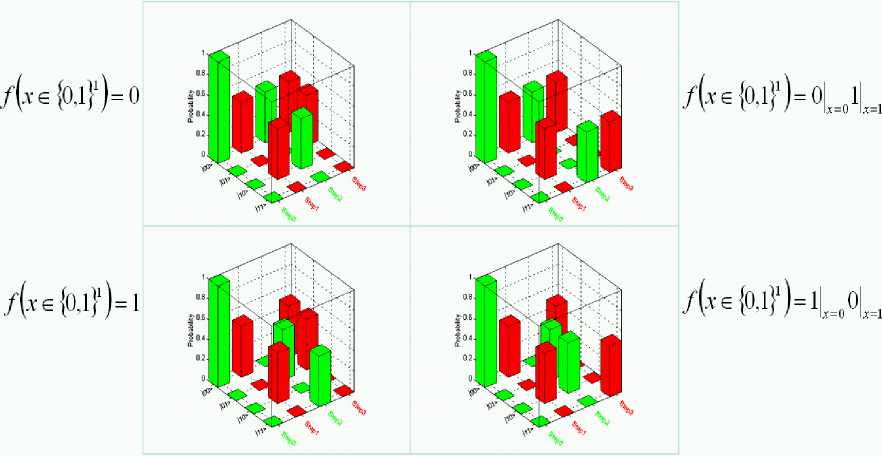
Figure 17. Deutsch quantum algorithm simulation: Algorithm 3d dynamics
Two-dimensional dynamic evolution of QAG for the case of constant function definition is shown in Fig. 18.
The case of balanced function definition the simulation result of QAG is shown in Fig. 19.
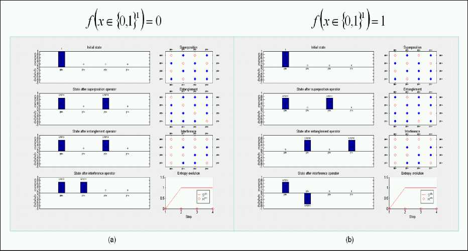
Figure 18. Deutsch quantum algorithm simulation: Algorithm 2d dynamics. Constant functions
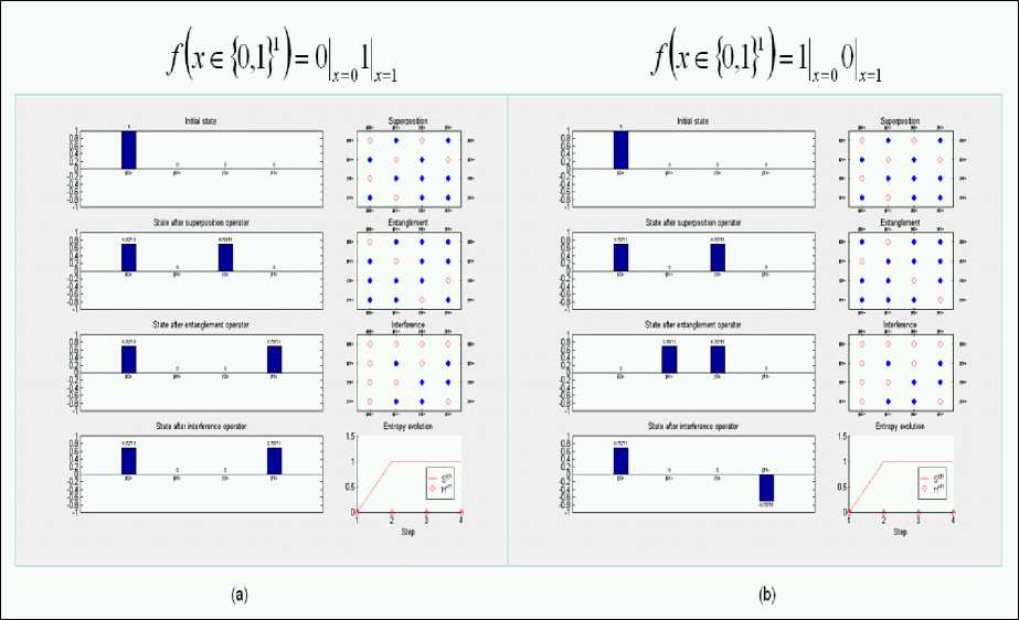
Figure 19. Deutsch quantum algorithm simulation: Algorithm 2d dynamics. Balanced functions
Figs 18 and 19 show also the entropy evaluation of the QAG for both cases.
These results are used for stopping criteria of the QA below.
Figs 20 and 21 show the results of final superposition measurement for definition of function property and its interpretation (decoding process), respectively.
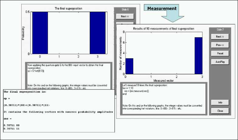
Figure 20. Deutsch’s quantum algorithm simulation, Step 5: Applying gate G to the input vector |00> and measurement
Output = IOO> Output = |01 >
Output = 111 >
Output = 110> nothing can be said, piobability 50% function f(x) is constant, probability 50% function f(x) is ballanced. probability 50% error, probability 0%
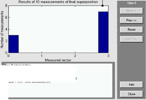
Result interpretation:
Result: Function is balanced
Figure 21. Deutsch’s quantum algorithm simulation, Step 6: Interpretation of results (decoding)
Deutsch-Jozsa’s algorithm
The Deutsch-Jozsa’s algorithm is based on the special form of its QAG. This example shows the importance of the structure of the matrix operator U F .
Deutsch-Jozsa's problem. Definition of Deutsch-Jozsa’s problem is stated as:
|
Input |
A constant or balanced function f:{0,1} n |
{0,1} |
|
Problem |
Decide if f is constant or balanced |
|
This problem is very similar to Deutsch’s problem, but it has been generalized to n > 1.
Fig. 22 shows the structure of the Problem and Fig. 23 shows the steps of gate design process.
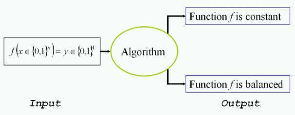
Figure 22. Deutsch-Jozsa’s QA: Problem definition
According to design steps on the Fig. 23 consider Step 0: the Encoder.
Step 0
Encoder. As a threshold matter, it is useful to deal with some special functions with n = 2 to illuminate various aspects of this algorithm. Then the general case with n = 2 is discussed, and finally a balanced or constant function is encoded in the more general situation n > 0.
|
N |
Definition of design step |
|
0 |
Step 0: Encoder Step 0.1: Injective function F building Step 0.2: Preparation of map table for entanglement operator Uf |
|
1 |
Step 1: Preparation of quantum operators Step 1.1: Preparation of superposition operator Step 1.2: Preparation of entanglement operator using information from step 0.2 Step 1.3: Preparation of interference operator Step 1.4: Quantum gate assembly |
|
2 |
Step 2: Algorithm execution Step 2.1: Application of superposition operator Step 2.2: Application of entanglement operator Step 2.3: Application of interference operator Step 2.4: Measurement and interpretation of the output |
Figure 23. Deutsch-Jozsa’s QA: Steps of the algorithm design
Consider the encoding steps process according to the structure in the Fig. 6.
-
A . Encoding a constant function with value 1. Consider the case:
n = 2, V x e { 0,1 } n : f ( x ) = 1 .
In this case, f map table is so defined:
|
x |
f ( x ) |
|
00 |
1 |
|
01 |
1 |
|
10 |
1 |
|
11 |
1 |
The encoder block takes f map table as input and encodes it into matrix operator U F , which acts inside of a complex Hilbert space.
Step 1
Function f is encoded into the injective function F , built according to the following statement:
F : { 0,1 } n + 1 ^ { 0,1 } n + 1: F ( x 0 , xv y 0 ) = ( x 0 , X 1 ,f ( x 0 , x i ) ф y 0 )
Then F map table is:
|
( x 0 , x 1 , y 0 ) |
F ( x 0 , x 1 , y 0 ) |
|
000 |
001 |
|
010 |
011 |
|
100 |
101 |
|
110 |
111 |
|
001 |
000 |
|
011 |
010 |
|
101 |
100 |
|
111 |
110 |
Step 2
Now encode F into U F map table using the rule:
Vte{0,1}n+1: Uf [?(t)]= t[F(t)], where тis the code map defined above. This means:
|
| x 0 x 1 y 0 > |
U F | x 0 x 1 y 0 > |
|
|000> |
|001> |
|
|010> |
|011> |
|
|100> |
|101> |
|
|110> |
|111> |
|
|001> |
|000> |
|
|011> |
|010> |
|
|101> |
|100> |
|
|111> |
|110> |
Here, ket notation is used to denote basis vectors.
Step 3
Starting from the map table of U F , calculate the corresponding matrix operator. This matrix is obtained using the rule:
[UF ]s= 1 Q UFj = |/) .
So, U F is the following matrix:
|
U F |
|000> |
|001> |
|010> |
|011> |
|100> |
|101> |
|110> |
|111> |
|
|000> |
0 |
1 |
0 |
0 |
0 |
0 |
0 |
0 |
|
|001> |
1 |
0 |
0 |
0 |
0 |
0 |
0 |
0 |
|
|010> |
0 |
0 |
0 |
1 |
0 |
0 |
0 |
0 |
|
|011> |
0 |
0 |
1 |
0 |
0 |
0 |
0 |
0 |
|
|100> |
0 |
0 |
0 |
0 |
0 |
1 |
0 |
0 |
|
|101> |
0 |
0 |
0 |
0 |
1 |
0 |
0 |
0 |
|
|110> |
0 |
0 |
0 |
0 |
0 |
0 |
0 |
1 |
|
|111> |
0 |
0 |
0 |
0 |
0 |
0 |
1 |
0 |
Using matrix tensor product, U F can be written as:
UF = I 0 I 0 C = 21 0 C where 0 is the tensor product, I is the identity matrix of order 2 and C is the NOT-matrix defined as:
. Matrix C flips a basis vector: in fact it transforms vector |0> into |1> and |1> into |0>.
If matrix U F is applied to the tensor product of three vectors of dimension 2, the resulting vector is the tensor product of the three vectors obtained applying matrix I to the first two input vectors and matrix C to the third.
Tensor product and entanglemen. Given m vectors v 1 ,.., v m of dimension 2 d 1,.., 2 dm and m matrix operators M 1 ,.., M m of order 2 d 1 x 2 d 1 ,.., 2 dm x 2 dm the following property holds:
( M 1 ® .. ® M m ) . ( V 1 ® .. ® v „ ) = M 1 • V 1 ® ... ® M m ■ v_n .
This means that, if a matrix operator can be written as the tensor product of m smaller matrix operator, the evolutions of the m vectors the operator is applied to are independent, namely no correlation is present among this vector. An important corollary is that if the initial state was not entangled, also the final state is not entangled. If, for example, UF = I ® I ® C then the structure of U f is such that first two vectors in the input tensor product are preserved (action of I ), whereas the third is flipped (action of C ). One can easily verify that this action corresponds to the constraints stated by U F map table.
-
B . Encoding a constant function with value 0 . Now consider the case:
n = 2
V x e { 0,1 } n : f ( x ) = 0
It is relatively easy to transform this map table into a matrix. Each vector is preserved. Therefore, the corresponding matrix is the identity matrix of order 23.
|
U F |
|000> |
|001> |
|010> |
|011> |
|100> |
|101> |
|110> |
|111> |
|
|000> |
1 |
0 |
0 |
0 |
0 |
0 |
0 |
0 |
|
|001> |
0 |
1 |
0 |
0 |
0 |
0 |
0 |
0 |
|
|010> |
0 |
0 |
1 |
0 |
0 |
0 |
0 |
0 |
|
|011> |
0 |
0 |
0 |
1 |
0 |
0 |
0 |
0 |
|
|100> |
0 |
0 |
0 |
0 |
1 |
0 |
0 |
0 |
|
|101> |
0 |
0 |
0 |
0 |
0 |
1 |
0 |
0 |
|
|110> |
0 |
0 |
0 |
0 |
0 |
0 |
1 |
0 |
|
|111> |
0 |
0 |
0 |
0 |
0 |
0 |
0 |
1 |
Using matrix tensor product, this matrix can be written as:
UF = I ® I 0 I = 21 0 I.
The structure of U F is such that all basis vectors of dimension 2 in the input tensor product evolve independently. No vector controls any other vector.
-
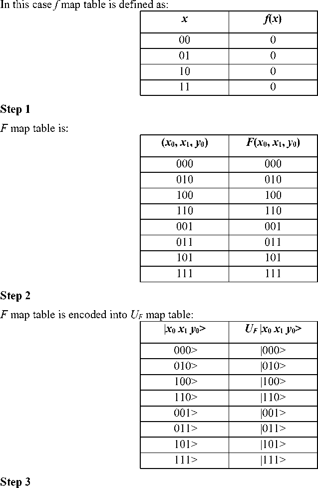
C . Encoding a balanced function. Consider now the balanced function:
n = 2, V ( x , ,...,X n ) e { 0,1 } n : f ( x ,,..., xn ) = x Ф---Ф x n .
In this case f map table is the following:
|
x |
f(x ) |
|
00 |
0 |
|
01 |
1 |
|
10 |
1 |
|
11 |
0 |
Step 1
The following map table calculated in the usual way represents the injective function F (where f is encoded into):
|
( x 0 , x 1 , y o ) |
F ( x o , x 1 , y o ) |
|
000 |
000 |
|
010 |
011 |
|
100 |
101 |
|
110 |
110 |
|
( x o , x 1 , y o ) |
F ( x o , x 1 , y o ) |
|
001 |
001 |
|
011 |
010 |
|
101 |
100 |
|
111 |
111 |
Step 2
Now encode F into U F map table:
|
| x 0 x 1 y 0 > |
U F | x 0 x 1 y 0 > |
|
|000> |
|000> |
|
|010> |
|011> |
|
|100> |
|101> |
|
|110> |
|110> |
|
|001> |
|001> |
|
|011> |
|010> |
|
|101> |
|100> |
|
|111> |
|111> |
Step 3
The matrix corresponding to U F is:
|
U F |
|000> |
|001> |
|010> |
|011> |
|100> |
|101> |
|110> |
|111> |
|
|000> |
1 |
0 |
0 |
0 |
0 |
0 |
0 |
0 |
|
|001> |
0 |
1 |
0 |
0 |
0 |
0 |
0 |
0 |
|
|010> |
0 |
0 |
0 |
1 |
0 |
0 |
0 |
0 |
|
|011> |
0 |
0 |
1 |
0 |
0 |
0 |
0 |
0 |
|
|100> |
0 |
0 |
0 |
0 |
0 |
1 |
0 |
0 |
|
|101> |
0 |
0 |
0 |
0 |
1 |
0 |
0 |
0 |
|
|110> |
0 |
0 |
0 |
0 |
0 |
0 |
1 |
0 |
|
|111> |
0 |
0 |
0 |
0 |
0 |
0 |
0 |
1 |
This matrix cannot be written as the tensor product of smaller matrices.
It can be written as a block matrix as follows:
|
U F |
|00> |
|01> |
|10> |
|11> |
|
|00> |
I |
0 |
0 |
0 |
|
|01> |
0 |
C |
0 |
0 |
|
|10> |
0 |
0 |
C |
0 |
|
|11> |
0 |
0 |
0 |
I |
This means that the matrix operator acting on the third vector in the input tensor product depends on the values of the first two vectors. If these vectors are |0> and |0>, for instance, the operator acting on the third vector is the identity matrix, if the first two vectors are |0> and |1> then the evolution of the third is determined by matrix C .
This operator creates entanglement , namely correlation among the vectors in the tensor product. One cannot represent such an operator as a tensor product of simpler operators such as I and C in the same manner as it was possible in case of entanglement operators of constant functions presented above.
-
D. General case with n = 2. Consider now a general function with n = 2.
In this general case f map table is the following:
x
f ( x )
00
f 00
01
f 01
10
f 10
11
f 11
with f i ∈ {0,1}, i =00,01,10,11.
If f is constant then ∃ y ∈ {0,1} ∀ x ∈ {0,1}2 : f ( x ) = y .
If f is balanced then |{ f i : f i = 0}|=|{ f i : f i = 1}|.
Step 1
Injective function F (where f is encoded) is represented by the following map table calculated in the usual way:
|
( x 0 , x 1 , y 0 ) |
F ( x 0 , x 1 , y 0 ) |
|
|
000 |
0 0 f 00 |
|
|
010 |
0 1 f 01 |
|
|
100 |
1 0 f 10 |
|
|
110 |
1 1 f 11 |
|
|
001 |
0 0 f 00 |
|
|
011 |
0 1 f 01 |
|
|
101 |
1 0 f 10 |
|
|
111 |
1 1 f 11 |
|
|
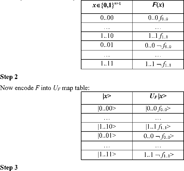
Step 2 Now encode F into U F map table: |
||
|
| x 0 x 1 y 0 > |
U F | x 0 x 1 y 0 > |
|
|
|000> |
|0 0 f 00 > |
|
|
|010> |
|0 1 f 01 > |
|
|
|100> |
|1 0 f 10 > |
|
|
|110> |
|1 1 f 11 > |
|
|
|001> |
|0 0 f 00 > |
|
|
|011> |
|0 1 f 01 > |
|
|
|101> |
|1 0 f 10 > |
|
|
|111> |
|1 1 f 11 > |
|
Step 3
The matrix corresponding to U F can be written as a block matrix with the following general form:
The structure of this matrix is such that, when the first two vectors are mapped into some other vectors, the null operator is applied to the third vector, generating a null probability amplitude for this transition. This means that the first two vectors are always left unchanged. On the contrary, operators M i ∈ { I , C } and they are applied to the third vector when the first two are mapped into themselves. If all M i coincide, operator U F encodes a constant function.
Otherwise, it encodes a non-constant function.
If |{ M i : M i = I }|=|{ M i : M i = C }| then f is balanced.
-
E . General case. Consider no w the general case n> 0. Input function f map table is the following:
with f i ∈ {0,1}, i ∈ {0,1} n .
If f is constant then ∃ y ∈ {0,1} ∀ x ∈ {0,1} n : f ( x ) = y .
If f is balanced then |{ f i : f i = 0}| = |{ f i : f i = 1}|.
Step 1
The map table of the corresponding injective function F is:
X € {0,1} n
f(x )
0..0
f 0..0
0..1
f 0..1
1..1
f… 1..1
The matrix corresponding to U F can be written as a block matrix with the following general form:
This matrix leaves the first n vectors unchanged and applies operator M i e { I, C } to the last vector. If all M i coincide with I or C , the matrix encodes a constant function and it can be written as nI ® I or nI ® C. In this case no entanglement is generated.
Otherwise, if the condition |{ M i : M i = I }|=|{ M i : M i = C }| is fulfilled, then f is balanced and the operator creates quantum correlation among vectors. It means that Deutsch-Jozsa’s QA needs bound amount of entanglement and can be efficiently simulated on classical computer.
Matrix tensor and dot powers. Given a matrix M denote its kth -power tensor product as: kM = M ® ... ® M ( k times ) . By contrast the k th -power dot product is: Mk = M ■ ... ■ M ( k times )
Quantum block. Matrix U F , the output of the encoder, is now embedded into the QAG of Deutsch-Jozsa’s algorithm. As with Deutsch’s algorithm, this gate is described using a quantum circuit in Fig. 24 (a).
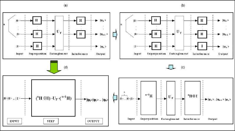
Figure 24. Deutsch-Jozsa’s quantum algorithm simulation: Circuit representation and corresponding gate design
Using Rule 3 (see Fig. 7), similar to the case of Deutsch’s QAG, compile the previous circuit into the one presented on the Fig. 24.
Now, consider operator U F in the case of constant and balanced functions. The structure of this operator strongly influences the structure of the whole gate. It is possible to analyze this structure in the case f is 1 everywhere, f is 0 everywhere and in the general case with n = 2.
The general form for the gate with n >0 is given below.
-
A . Constant function with value. 1. If f is constant and its value is 1, matrix operator U F can be written as nI ® C. This means, as it is stated by Rule 1 in Fig. 7, that U f can be decomposed into n +1 smaller operators acting concurrently on the n +1 vectors of dimension 2 in the input tensor product.
The resulting circuit representation is shown according to Fig. 24 in Fig. 25.
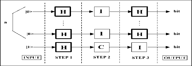
Figure 25. Constant Function with Value 1 — First Circuit
Now use Rule number 2 from Fig. 7 and find the sub-gate acting on every vector of dimension 2 in input. The result of this operation is shown in Fig. 26.
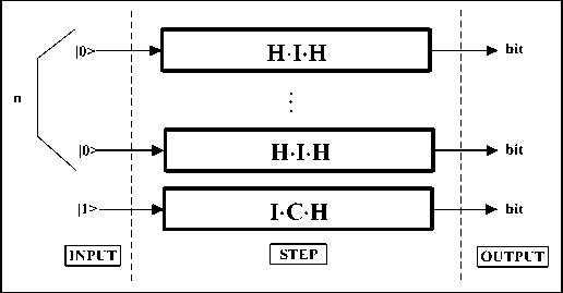
Figure 26. Constant Function with Value 1 — Second Circuit
Observe that every vector in input evolves independently from other vectors. This is because operator U F doesn’t create any correlation. So, the evolution of every input vector can be analyzed separately.
This circuit can be written in a simpler way as shown in Fig. 27, observing that M ⋅ I = M.
It can be show that H 2 = I.
Therefore the circuit is rewritten in this way as shown in Fig. 28.
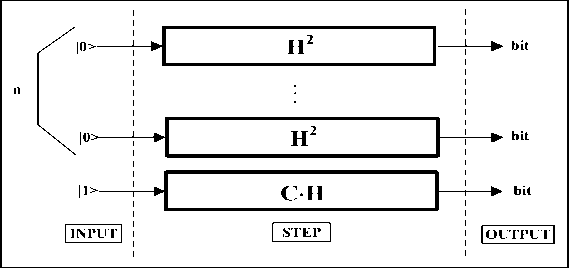
Figure 27. Constant Function with Value 1 — Third Circuit
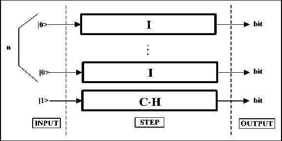
Figure 28. Constant Function with Value 1 — Fourth Circuit
Consider now the effect of the operators acting on every vector:
I 10)=10),
C ■ я | i=- *°У1 •
Using these results in rule number 4 of Fig. 7 and applying Rule number 3 of Fig. 7, yields following circuit representation as shown on the Fig. 29 as the particular case of the structure shown in Fig. 24.
|
---► |0> |
||||
|
|0> n |
. . . |
----► |0> |
||
|
|0> |
||||
|
|1> |
► |
C - H |
k |0>-|1> 2 1/2 |
|
|
INPUT |
STEP |
OUTPUT |
Figure 29. Constant Function with Value 1 — Fifth Circuit
It is easy to see that, if f is constant with value 1, the first n vectors are preserved.
-
B. Constant function with value. 0. A similar analysis can be repeated for a constant function with value 0. In this situation U f can be written as nI ® I and the final circuit is shown on the Fig. 3.30. Also in this case, the first n input vectors are preserved. So, their output values after the QAG has acted are still |0>.
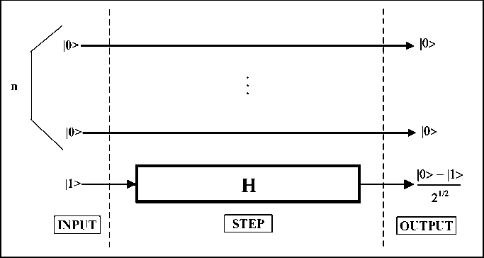
Figure 30. Constant Function with Value 0 — Final Circuit
-
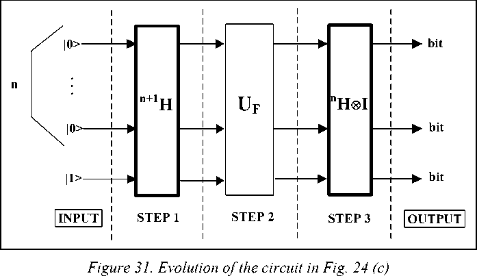
C. General case ( n = 2). The gate implementing Deutsch-Jozsa’s algorithm in general case is obtained operating on the circuit of Figs 24c and 24d, with Rules 1 and 2 defined in Fig. 7. This is the circuit evolution as shown on the Figs 31and 32.
If n = 2, U F has the following form:
U F
|00>
|01>
|10>
|11>
|00>
M 00
0
0
0
|01>
0
M 01
0
0
|10>
0
0
M 10
0
|11>
0
0
0
M 11
where M i ∈ { I , C }, i = 00,01,10,11.
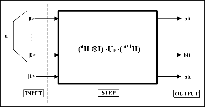
Figure 32. Deutsch-Jozsa’s quantum gate
Calculate the QG G= ( 2H ⊗ I ) ⋅ U F ⋅ ( 2+1H ) in this case:
|
3H |
|00> |
|01> |
|10> |
|11> |
|
|00> |
H /2 |
H /2 |
H /2 |
H /2 |
|
|01> |
H /2 |
- H /2 |
H /2 |
- H /2 |
|
|10> |
H /2 |
H /2 |
- H /2 |
- H /2 |
|
|11> |
H /2 |
- H /2 |
- H /2 |
H /2 |
|
2 H 0 I |
|00> |
|01> |
|10> |
|11> |
|
|00> |
I /2 |
I /2 |
I /2 |
I /2 |
|
|01> |
I /2 |
- I /2 |
I /2 |
- I /2 |
|
|10> |
I /2 |
I /2 |
- I /2 |
- I /2 |
|
|11> |
I /2 |
- I /2 |
- I /2 |
I /2 |
|
U f • 3 H |
|00> |
|01> |
|10> |
|11> |
|
|00> |
M 00 H /2 |
M 00 H /2 |
M 00 H /2 |
M 00 H /2 |
|
|01> |
M 01 H /2 |
- M 01 H /2 |
M 01 H /2 |
- M 01 H /2 |
|
|10> |
M 10 H /2 |
M 10 H /2 |
- M 10 H /2 |
- M 10 H /2 |
|
|11> |
M 11 H /2 |
- M 11 H /2 |
- M 11 H /2 |
M 11 H /2 |
|
G |
|00> |
|01> |
|10> |
|11> |
|
|00> |
(M 00 +M 01 +M 10 +M 11 )H/4 |
(M 00 -M 01 +M 10 -M 11 )H/4 |
(M 00 +M 01 -M 10 -M 11 )H/4 |
(M 00 -M 01 -M 10 +M 11 )H/4 |
|
|01> |
(M 00 -M 01 +M 10 -M 11 )H/4 |
(M 00 +M 01 +M 10 +M 11 )H/4 |
(M 00 -M 01 -M 10 +M 11 )H/4 |
(M 00 +M 01 -M 10 -M 11 )H/4 |
|
|10> |
(M 00 +M 01 -M 10 -M 11 )H/4 |
(M 00 -M 01 -M 10 +M 11 )H/4 |
(M 00 +M 01 +M 10 +M 11 )H/4 |
(M 00 -M 01 +M 10 -M 11 )H/4 |
|
|11> |
(M 00 -M 01 -M 10 +M 11 )H/4 |
(M 00 +M 01 -M 10 -M 11 )H/4 |
(M 00 -M 01 +M 10 -M 11 )H/4 |
(M 00 +M 01 +M 10 +M 11 ) H/4 |
Now, consider the application of G to vector |001>:
G |001) = 1H ® ( M 00 + M 01 + M io + M 11 ) H 1 + 1^1 ® ( M 00 - M 01 + M 10 - M 11 ) H 1 +
+1|10> ® ( M 00 + M 01 - M 10 — M 11 ) H |1 +^l ® ( M 00 — M 01 — M 10 + M 11 ) H 11
Consider the operator ( M 00 + M 01 + M 10 + M 11 ) H under the hypotheses of balanced functions M i e { I , C }and |{ M i : M i = I }| = |{ M i : M i = C }|. Then:
|
M 00 + M 01 + M 10 + M 11 |
|0> |
|1> |
|
|0> |
2 |
2 |
|
|1> |
2 |
2 |
|
( M 00 + M 01 + M 10 + M 11 ) H/ 4 |
|0> |
|1> |
|
|0> |
1/21/2 |
0 |
|
|1> |
1/21/2 |
0 |
Thus:
1 (M00 + M0! + Mw + Mn) H |1) = 0 .
This means that the probability amplitude of vector |001> of being mapped into a vector |000> or |001> is null.
Consider now the operators:
( M 00 + M 01 + M 10 + M 11 ) H
( M 00 - M 01 + M io - M 11 ) H
( M oo + M oi - M io - M ii ) H
(M00-M01-M10+M11)H under the hypotheses Vi: Mi = I, which holds for constant functions with values 0:
|
M 00 + M 01 + M 10 + M 11 |
|0> |
|1> |
|
|0> |
4 |
0 |
|
|1> |
0 |
4 |
|
( M 00 + M 01 + M 10 + M 11 ) H/ 4 |
|0> |
|1> |
|
|0> |
1/21/2 |
1/21/2 |
|
|1> |
1/21/2 |
-1/21/2 |
|
M 00 - M 01 + M io - M ii |
|0> |
|1> |
|
|0> |
0 |
0 |
|
|1> |
0 |
0 |
|
M oo + M oi - M io - M ii |
|0> |
|1> |
|
|0> |
0 |
0 |
|
|1> |
0 |
0 |
|
M oo - M oi - M io + M ii |
|0> |
|1> |
|
|0> |
0 |
0 |
|
|1> |
0 |
0 |
Using these calculations, the following results are obtained:
1 ( M 00 - M 01 + M 10 - M ii ) H |i) = 0,
1 ( M 00 + M 0i - M 10 - M ii ) H |i) = 0,
1 ( M 00 - M 0i - M ю + M ii ) H |i) = 0.
This means that the probability amplitude of vector |001> of being mapped into a superposition of vectors |010>, |011>, |100>, |101>, |110>, |111> is null. The only possible output is a superposition of vectors |000> and |001>, as shown before using circuits. A similar analysis can be developed under the hypotheses V i : M i = C .
It is useful to outline the evolution of the probability amplitudes of every basis vector while operator 3 H , U F and 2 H ⊗ I are applied in sequence, for instance when f has constant value 1. This is shown in Fig. 33.
|
1 0,5 0 -0,5 -1 |
|||
|
|000> |001> |010> |011> |100> |101> |110> |111> |
|||
Figure 33 (a). Input probability amplitudes
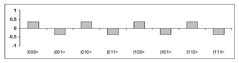
Figure 33 (b). Probability amplitudes after Step 1
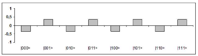
Figure 33 (с). Probability amplitudes after Step 2
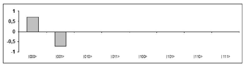
Figure 33 (d). Probability amplitudes after Step 3
Operator 3 H in Fig. 33 (b) puts the initial canonical basis vector |001> into a superposition of all basis vectors with the same (real) coefficients in modulus, but with positive sign if the last vector is |0>, negative otherwise.
Operator U F in Fig. 33 (c) in this case doesn’t create correlation: it flips the third vector independently from the values of the first two vectors.
Finally, 2 H ⊗ I in Fig. 33 (d) produces constructive interference: for every basis vector | x 0 x 1 y 0 > it calculates its output probability amplitude α ’ x x y as the summation of the probability amplitudes of all basis vectors in the form | x 0 x 1 y 0 > in the input superposition, all with the same sign if | x 0 x 1 > = |00>, otherwise changing the sign of exactly the middle of the probability amplitudes. Since, in this case, the vectors in the form | x 0 x 1 0> have the same (negative real) probability amplitude and vectors in the form | x 0 x 1 1> have the same (positive real) probability amplitude, when | x 0 x 1 > = |00>, probability amplitudes interfere positively. Otherwise the terms in the summation interfere destructively annihilating the result.
D. General case ( n > 0). In the general case n > 0, U F has the following form:
Calculate t he QAG G= ( nH ® I) ■ U f ■ ( n+ 1 H :
|
n+1H |
|0..0> |
… | j > |
|1..1> |
|
|0..0> |
H /2 n /2 |
… H /2 n /2 |
H /2 n /2 |
|
| i > |
H /2 n /2 |
_ (-1) ij H /2 n /2 |
(-1) i' t1-1) H /2 n /2 |
|
|1..1> |
H /2 n /2 |
_ (-1)(1-1) ■ jH /2 n /2 . |
(-1)(i-D -d-D h /2 n /2 |
Here the binary string operator, which represents the parity of the AND bit per bit between two strings, is used.
Priority of bit per bit AND Given two binary strings x and y of length n , define:
x ■ y = xx ■ y Ф x 2 ■ y 2 Ф ... Ф xn ■ yn
The symbol « ■ » used between two bits is interpreted as the logical AND operator.
It can be shown that the matrix n +1 H really has the described form. It can be shown that:
L H 1 ij
I - 1 ) 'v
2 n /2 ,
The proof is by induction: n = 1:
Г 1 h 1
L J o,o
Г 1 H 1
L -11,0
1 ( - 1 ), 0 ), 1 )
2 1/2 = 2 1/2
Г 1 H 1

- 1 ( - 1 )IW)
2 1/2 21/2
n > 1:

' 0, j 0
= 2? [ n - 1 H ] - , ,
1 ( _ i )- j _( _ 1 ) < ' 0 >0 0 )
1/2 ^( ” - 1 ) /2 ^” /2
Г•-1H1 (-i)'j (-1)('°' 21/2 L H ]',j 21/2 2(”-1)/2 2”/2 r”H L=2 L ”-1H L= L ”H L=- ,. L -1H L 1 (-1)'-j (-1)('1>(j0) 1/2 ^(”-1'/2 2”/2 _ (-1) -j (-1)™j1 ^ 1/2 ^(”-1)/2 2”/2 Matrix n+1H is obtained from nH by tensor product. Similarly, matrix nH ® I is calculated: nH®I |0..0> … |j> |1..1> |0..0> I/2n/2 … I/2n/2 I/2n/2 |i> I/2n/2 „. (-1)ijI/2n/2 (-1)i' (1-1)I/2n/2 |1..1> I/2n/2 _ (-1)(1-1) jI/2n/2 _ (-1)(1..1) -(1..1)I/2n/2 Uf -n+1H |0..0> … |j> … |1..1> |0..0> M0..0H/2n/2 … M0..0H/2n/2 … M0..0H/2n/2 |i> MiH /2n/2 … (-1) ij' MiH/2n/2 . (-1) i' (1..1) MiH/2n/2 |1..1> M1..1H/2n/2 … (-1)(1..1)j' M1..1 H/2n/2 . (-1)(1..1) -(1..1) m1..1 h/2n/2 Only the first column of gate G is calculated since this operator is applied exclusively to input vector |0…01> and so only the first column is involved. G |0..0> … |0...0> (M0..0+..+Mi+..+M1..1)H/2n … |i> ( S;e{0,1} n (-1)ijMj ) H/2n |1...1> ( S jE{0,1} n (-1)(1..1) jMj) H/2n ... Now consider the case of f constant. This means that all matrices Mi are identical. This implies: Jn- (2 J(-^-'M,) H=0, In this summation the number of +1 equals the number of –1. Therefore, the input vector |0…01> is mapped into a superposition of vectors |0…00> and |0…01> as shown using circuits. If f is balanced, the number of Mi = I equals the number of Mi = C. This implies: —(У mAh =—(2n-11+2n-1Ch =1 1 2nx^j j/ 2n\ ) 21 H = 2V2 [1 1JL1 1 1 1 -1]" v2 [1 And therefore: . (2,M,) H 1=0. This means that input vector |0…01>, in the case of balanced functions, cannot be mapped by the QAG into a superposition containing vectors |0…00> or |0…01>. The quantum block terminates with measurement. The above results show the possible outputs of measurement and their probabilities: Superposition of Basis Vectors (Before Measurement) Result of Measurement Vector Probability Constant functions: |0..00> ||a0||2 G 0_O1>=0..O>®(aD0>+a1|1>) |0..01> ||a1||2 Balanced functions: G|0...01>=Sie{0,1}n - {0..00,0..01} ai |i> Vie{0,1}n-{0..00, 0..01}:|i> ||a/1|2 The set A -B is given by all elements of A, unless those elements belonging to B too. This set is sometimes denoted as A/B. The quantum block is repeated only one time in Deutsch-Jozsa’s algorithm. So, the final collection is made only by one vector. Decoder. As in Deutsch’s algorithm, when the final basis vector has been measured, one must interpret it in order to decide if f is constant or balanced. If the resulting vector is |0…0> it is known that the function was constant, otherwise it is balanced. In fact gate G produces a vector such that, when it is measured, only basis vectors |0…00> and |0…01> have a non-null probability amplitude exclusively in the case f is constant. Besides, if f is balanced, these two vectors have null coefficients in the linear combination of basis vectors generated by G. In this way, the resulting vector is decoded in order to answer Deutsch-Jozsa’s problem: Resulting Vector (after measurement) Answer |0…00> f is constant |0…01> f is constant otherwise f is balanced Computer design process of Deutsch-Jozsa QAG (D.–J. QAG) and simulation results. Consider the design process of the Deutsch-Josa QAG according to the steps represented in Fig. 23. For step 0 (encoding), case n = 3 , examples of constant and balanced functions encoding are shown in Figs 34 and 35. Figure 34. Deutsch-Jozsa’s QA: Step 0. Constant functions encoding. Order n = 3 Figure 35. Deutsch-Jozsa’s QA: Step 0. Balanced functions encoding. Order n = 3 For step 1 in Fig. 23, the example of quantum operator preparation such as superposition operator in Fig. 36 is shown. Figure 36. Deutsch-Jozsa’s QA: Step 1.1. Preparation of quantum operators: Superposition operator Figs 37-40 shows the step 1.2 from Fig. 23 as the preparation of entanglement operators: For a constant function: f (e{0,1}3 = 0) and f (e{0,1}3 = 1) as shown in Figs 37 and 38; For a balanced function: f (®{0.1}3 = 11 x >011 o|xs0,,) and f ^{0.1)3 = x = {010,011,110,111}^ x = {000,001,100,101} v as shown in Figs 39 and 40 respectively. Figure 37. Deutsch-Jozsa’s QA: Step 1.2. Preparation of quantum operators: Entanglement operator Figure 38. Deutsch-Jozsa’s QA: Step 1.2. Preparation of quantum operators: Entanglement operator Figure 39. Deutsch-Jozsa’s QA: Step 1.2. Preparation of quantum operators: Entanglement operator Figure 40. Deutsch-Jozsa’s QA: Step 1.2. Preparation of quantum operators: Entanglement operator Step 1.3 in Fig. 23 shows the preparation of the interference operator and is shown in Fig. 41. Comparison between superposition and interference operators is shown in Fig. 42. Figure 41. Deutsch-Jozsa’s QA: Step 1.3. Preparation of quantum operators: Interference operator Figure 42. Deutsch-Jozsa’s QA: Superposition and interference operators The evolution of gate design process from Fig. 23 is shown in Fig. 43. Figure 43. Deutsch-Jozsa’s QA: Step 1.4. Quantum gate assembly Step 1.4 from Fig. 23 as QAG assembly for design cases is shown in Fig. 44. Figure 44. Deutsch-Jozsa’s QA: Step 1.4. Assembled quantum gates Figs 45 and 46 show the results of algorithm gate execution for constant and balanced functions respectively (corresponding to step 2 from Fig. 23). (a) (b) Figure 45. Deutsch-Jozsa’s QA: Step 2. Algorithm execution: Constant functions (a) (b) Figure 46. Deutsch-Jozsa’s QA: Step 2. Algorithm execution: Balanced functions Fig. 47 shows the 3D result of amplitude probability evolution for Deutsch-Jozsa’s QA execution. Figure 47. Deutsch-Jozsa’s QA: Step 2. Algorithm execution 3d dynamics: Probability amplitudes Fig. 48 shows the 3D result of probability evolution of this QA. Fig. 48. Deutsch-Jozsa’s QA: Step 2. Algorithm execution 3d dynamics: Probabilities Result interpretation (corresponding to step 2.4 from Fig. 23) is shown in Fig. 49. Figure 49. Deutsch-Jozsa’s QA: Step 2.4 Result interpretation In Deutsch-Jozsa’s QA, the mathematical and physical structures of the interference operator (nH ® I) differ from its superposition operator (n+1H). The interference operator extracts the qualitative information about the property (constant or balanced property of function f) with operator nH , and separate this property qualitatively with operator I. Deutsch-Jozsa’s QA is a decision making algorithm. For the case of Deutsch-Jozsa’s QA only one iteration is needed without estimation quantitatively the qualitative property of function f and with error probability 0.5 of successful result. It means that the Deutsch-Jozsa QA is a robust QA. The superposition operator organizes the quantum massive parallel computation process and robust extraction of function property is provided by the entanglement operator. The next section illustrates the Simon’s QA and the role of the interference operator in the searching problem. Simon’s algorithm Simon’s algorithm is now illustrated using circuits and pointing out the role of interference. Simon's problem. Simon’s problem is formulated as follows: Input f {0,1}n ^{0,1}n: 3se {0,1}n-{0..0}:Vx,ye {0,1}n:f(x) = f(y) о (x = y vx = y©s) Problem Find s Encoder. As for the Deutsch-Jozsa’s algorithm, firstly consider some special cases. A. Introductory example. Consider the case: n = 2, f (00) = 00, f (01) = 01, 5 = 11. Then, the f map table is: (x0, x1) f(x0, x1) 00 00 01 01 10 01 11 00 Step 1 Function f is encoded into the injective function F built in the usual way: F: {0,1}n+n ^{0,1}n+n such that F (x 0, x1,..,xn -1, y 0, У1,.., Уп -1 ) = ( x0, x1,..,xn-1,f(x0, x1,..,xn-1 )©( y 0, У1,.., Уп -1)) This is the F map table: (x0,.., xn-1, y0,.., yn-1) F(x0,.., xn-1, y0,.., yn-1) 0000 0000 0100 0101 1000 1001 1100 1100 0001 0001 0101 0100 (x0,.., xn-1, y0,.., yn-1) F(x0,.., xn-1, y0,.., yn-1) 1001 1000 1101 1101 0010 0010 0110 0111 1010 1011 1110 1110 0011 0011 0111 0110 1011 1010 1111 1111 Step 2 Now encode F map table into UF map table. As usually, the rule is: ∀t∈{0,1}n+n: UF [τ(t)]= τ[F(t)], where τ is the code map defined by Eq. (2) above. This means: |x0.. xn-1 y0.. yn-1> UF|x0.. xn-1 y0.. yn-1> |0010> |0010> |0110> |0111> |1010> |1011> |1110> |1110> |0011> |0011> |0111> |0110> |1011> |1010> |1111> |1111> Step 3 Using the rule: [UF ]ij = 1 ⇔ UF I j)=i) calculate UF as a block matrix: UF |00> |01> |10> |11> |00> I⊗I 0 0 0 |01> 0 I⊗C 0 0 |10> 0 0 I⊗C 0 |11> 0 0 0 I⊗I This matrix preserves the first two vectors in the input tensor product vector. It preserves the last two when the first two vectors are |0> and |0> or |1> and |1>. It preserves the third vector, but it flips the fourth, when the first two vectors are |0> and |1> or |1> and |0>. Observe that the block matrix in cell (i, i) is identical to the block matrix in cell (i⊕s, i⊕s), where i is the binary label of the vector marking the matrix row and column of the cell. B. General case with n = 2. In general, if n = 2, repeating steps 1, 2 and 3 as for Deutsch-Jozsa’s algorithm, the general operator UF is obtained in the following form: UF |00> |01> |10> |11> |00> M00 0 0 0 |01> 0 M01 0 0 |10> 0 0 M10 0 |11> 0 0 0 M11 where Mi∈{I⊗I, I⊗C, C⊗I, C⊗C} and Mi=Mj⇔(j=i∨j=i⊕s). C. General case. Generalizing the results obtained in the previous examples and reasoning like in Deutsch-Jozsa’s algorithm, one can find the structure of UF for Simon’s algorithm too. The final matrix is: UF |0..0> |0..1> … |1..1> |0…0> M0...0 0 … 0 |0…1> 0 M0…1 … 0 |1...1> 0 0 … ... 0 M1...1 where Mi = P1⊗…⊗Pn , Pk∈{I, C}, k=1,…,n and Mi = Mj⇔(j=i∨j=i⊕s). Note that the column labels are basis vectors of dimension n (not 2n). Quantum block In Fig. 50 (a) shows the circuit describing Simon’s QG. Figure 50. Simon’s quantum algorithm simulation: Circuit representation and corresponding gate design Using the transformation rules defined in Fig. 23 this circuit is complied into the corresponding gate. Fig. 50 (d) shows Simon's QAG. To calculate this gate and establish what output vector it produces, it is first useful to deal with the introductory example of Section A, passing then to the general case with n = 2. Finally, the gate structure is described in the general situation (n > 0). A. Introductory example. In the case considered before (n = 2, f(00) = 00, f(01) = 01, s = 11), the QAG assumes this form: G=(nH⊗nI) ⋅UF⋅(nH⊗nI) where UF has been calculated in Section A, Step 2. Start finding matrix 2H ®21, using the results about the tensor power of matrix H obtained in previous section. 2H®21 |00> |01> |10> |11> |00> 2I/2 2I/2 2I/2 2I/2 |01> 2I/2 - 2I/2 2I/2 - 2I/2 |10> 2I/2 2I/2 - 2I/2 - 2I/2 |11> 2I/2 - 2I/2 - 2I/2 2I/2 Recall matrix UF and calculate G: UF |00> |01> |10> |11> |00> 2I 0 0 0 |01> 0 I®C 0 0 |10> 0 0 I®C 0 |11> 0 0 0 2I Uf • (2H ®2I) |00> |01> |10> |11> |00> 2I/2 2I /2 2I/2 2I/2 |01> I® C/2 -1® C/2 I® C/2 -1® C/2 |10> I® C/2 I® C/2 -1® C/2 -1® C/2 |11> 2I/2 - 2I/2 - 2I/2 2I/2 G |00> |01> |10> |11> |00> (21+1® C )/2 0 0 (21-1® C )/2 |01> 0 (21+1® C )/2 (21-1® C )/2 0 |10> 0 (21-1® C )/2 (21+1® C )/2 0 |11> (21-1® C )/2 0 0 (21+1® C )/2 With G from (3.2) having this structure, apply it to vector |0000> to obtain the following result: (21 +1 ® C) (21 -1 ® C) G10000) = 100)2-----------L100) +111)2-----------2100). This means: G о»00)=|W (I °°)+101))+^Н (I °°)-I 01). If the output vector is measured, one can obtain only 4 possible results: |0000>, |0001>, |1100> and |1101>. Encode back into their binary labels the values of the first two basis vectors of dimension 2 in the output tensor product: these labels are 00 or 11. Then solve the system: '(00)-(ti12) = 0 fo-tx ©0-t2 = 0 <(11)-(txq) = 0 ^J1-tx © 1-12 = 0 tx * 0, t2 * 0 t1 * 0,t2 * 0 0 © 0 = 0 ^ < tx © t2 = 0 ^ tx * 0, t2 * 0 tx © t2 = 0 f tx = 1 tx * 0, t2 * 0 Ц t2 = 1" Since s=(11), then s=(t1 , t2). Therefore, s can be calculated as the solution of the system: t 00). s = 0 . (П).s = 0 s *( 0,0) B. General case with n = 2. In the general case with n=2, matrix UF has the form: UF |00> |01> |10> |11> |00> M00 0 0 0 |01> 0 M01 0 0 |10> 0 0 M10 0 |11> 0 0 0 M11 where Mie {I©I, I©C, C©I, C©C} and Mi = Mj о (j'=i v j=i©s). Using matrix 2H ©21 calculated above, obtain:_____________ Uf - (2H ©21) |00> |01> |10> |11> |00> M00/2 M00/2 M00/2 M00/2 |01> M01/2 -M01/2 M01/2 -M01/2 |10> M10/2 M10/2 -M10/2 - M10/2 |11> M11/2 -M11/2 -M11/2 M11/2 G |00> |01> |10> |11> |00> (M00+M01+M10+M1 1)/4 (M00-M01+M10-M11)/4 (M00+M01-M10-M11)/4 (M00-M01-M10+M11)/4 |01> (M00-M01+M10-M11)/4 (M00+M01+M10+M1 1)/4 (M00-M01-M10+M11)/4 (M00+M01-M10-M11)/4 |10> (M00+M01-M10-M11)/4 (M00-M01- M10+M11)/4 (M00+M01+M10+M1 1)/4 (M00-M01+M10-M11)/4 |11> (M00-M01- M10+M11)/4 (M00+M01-M10-M11)/4 (M00-M01+M10-M11)/4 (M00+M01+M10+M 11)/4 Now, consider the following cases: ( i) s = 01; (ii) s = 10; (iii) s = 11. In the first case M00=M01≠M10=M11. This means: G01 |00> |01> |10> |11> |00> (M00+M10)/2 0 (M00-M10)/2 0 |01> 0 (M00+M10)/2 0 (M00-M10)/2 |10> (M00-M10)/2 0 (M00+M10)/2 0 |11> 0 (M00-M10)/2 0 (M00+M10)/2 In the second case M00=M10 ≠M01=M11. This means: G10 |00> |01> |10> |11> |00> (M00+M01)/2 (M00-M01)/2 0 0 |01> (M00-M01)/2 (M00+M01)/2 0 0 |10> 0 0 (M00+M01)/2 (M00-M01)/2 |11> 0 0 (M00-M01)/2 (M00+M01)/2 Finally, in the third case M00=M11≠M01=M10. This means: G11 |00> |01> |10> |11> |00> |01> |10> |11> (M00+M01)/2 0 0 (M00-M01)/2 0 (M00+M01)/2 (M00-M01)/2 0 0 (M00-M01)/2 (M00+M01)/2 0 (M00-M01)/2 0 0 (M00+M01)/2 Consider the ap lication of G01, G10 and G11 to vector |0000> in the three cases: Case s Output vector: Gs|0000> 1 01 G01|0000>=1/2 |00>(M00+M10)|00> + 1/2 |10>(M00-M10)|00> 2 10 G10|0000>=1/2 |00>(M00+M01)|00> + 1/2 |01>(M00-M01)|00> 3 11 G11|0000>=1/2 |00>(M00+M01)|00> + 1/2 |11>(M00-M01)|00> Measure the output vector in these three cases and encode back into binary values the first two basis vectors in the tensor product, to obtain the following result: Case s Binary Values (FROM THE FIRST TWO VECTORS) Probabilities 1 01 (a, b)=(0,0) (a, b)=(1,0) 0.5 0.5 2 10 (a, b)=(0,0) (a ,b)=(0,1) 0.5 0.5 3 11 (a, b)=(0,1) (a, b)=(1,1) 0.5 0.5 Note that (a, b) ⋅s = 0 where a and b are the binary values from the first two vectors. The equations so generated let us find s as the solution of the corresponding system. C. General case (n > 0). Now consider a general positive value for number n. The operator UF is: The first column of the final gate has the following form: G |0..0> |0..0> (M0..0+..+Mi+..+M1..1)/2n … |i> ( Σj∈{0,1}n (-1)i⋅jMj )/2n … |1..1> ( Σ j∈{0,1}n (-1)(1..1) ⋅jMj )/2n … Operator nH⊗nI is built from operator nH: nH ⊗nI |0..0> |0..1> … |j> … |1..1> |0..0> nI/2n/2 nI/2n/2 … nI/2n/2 … nI/2n/2 |0..1> nI/2n/2 - nI/2n/2 … (-1)(0..1) ⋅j(nI/2n/2) … - nI/2n/2 |i> nI/2n/2 (-1)i⋅(0..1) (nI/2n/2) … (-1)i⋅j (nI/2n/2) … (-1) i⋅(1..1) (nI/2n/2) |1..1> nI/2n/2 - nI/2n/2 … (-1)(1..1)⋅j (nI/2n/2) … (-1)(1.. 1) ⋅(1..1) (nI/2n/2) UF⋅(nH⊗nI) |0..0> … |j> … |1..1> |0..0> M0..0/2n/2 … M0..0/2n/2 … M0..0/2n/2 |i> Mi/2n/2 … (-1)i⋅j Mi/2n/2 … (-1)i⋅(1..1) Mi/2n/2 |1..1> M1..1/2n/2 … (-1)(1..1) ⋅j M1..1/2n/2 … (-1)(1..1) ⋅(1..1) M1..1/2n/2 The interference operator (n H⊗n I) creates the following term: 1n ∑ (-1)i⋅jMj. 2 j∈{0,1}n Since Mh = Mk о (h = k v h = k*s), then this term may be written as: Z ИХ = 2 j e{0,1} } 1k£[(-1)“ ■1 1‘*‘)]Mk = 1 Z 11 [‘ ■ '"‘]Mk • 2k e 5 2k e 5 where S is such that: —3x,y e 5: x * s = y —3x,y e{0,1}n - 5 : x * s = y. The gate can be rewritten in this way: G |0..0> … |0…0> 2 keS (-1)(0-0)^k ||-(-l)"/ '" ^s ] Mk /2 n -^ |i> Zk es(-1)ik [1+(-1)is ] Mk /2 n |1…1> 2keS (-1)(1-1)k[1+(-1)"1.1)"]Mk/2n . The term [1+ (- 1) is] is 0 if and only if i • s = 1. So, only those cells in the column that are labeled by li> such that i s = 0 are non-null. This means that: G| 0..0°..0) = -3 £ |f). 2 i e{0,1} n: is=0 The quantum block ends with measurement, which therefore produces a basis vector |i> such that i • s = 0. Thus, the interference operator (nH ® nI) is created the important component of final result and with the entanglement operator and a measurement process can extract this final result. In this case, the interference operator (nH ® nI) extracts the qualitative property of the function f using operator (nH) and estimates quantitatively this property as a solution number with operator (nI). With tensor product (®)the interference operator (nH ® nI) joins both possibilities in one automation operation. Simon’s QA is the search algorithm and this property is described by specific structure of interference operator. Operator (nH) from interference operator (nH ® I) in Deutsch-Jozsa’s QA created the distribu tion of probability amplitude with the same amplitude of probability |a0 | = |a I = ; the measurement with the ancillae qubit as -j=(| 0) -| 1))® I extracts only the qualitative information about the function f, and 2 gives sufficient and necessary values of probability 0.5 for the separation of solutions in decision-making algorithm. The quantum block for this QA is repeated only one time and the final collection is made only one basic vector. For state vector i of Deutsch-Jozsa’s QA the estimator of amplitude of probability is: £ £ (-1)-M, H. I 2 je{0,1}n J The operator H in this operator plays the role of the destructive interference for ancillary qubit: H | -U[| 0) -1J | = |0) and realize toss and coin procedure of random measurement. The different signs к V2 ) of amplitude probability in ancillary qubit with identity operator I guarantee the recognition the so- lution with toss and coin procedure of measurement that is necessary and sufficient conditions for successful result of quantum computing. In the case of Simon’s QA the estimator of amplitude of probability in state vector i is as follows: Choice of solution k e 5 k e 5 + (-1)1®' Mk, Quantitavesolution estimator where S is such that include almost quantitative information about the solutions. The estimator of amplitude probability in Simon’s QA constructively distributed the amplitude of probability: increase the amplitude for «good» solution with quantitative estimation of this solution and decrease other amplitudes of solution probability. In Simon’s QA the role of interference is different than in Deutsch-Jozsa’s QA while this operator extract the qualitative information about the solution and estimate quantitatively this solutions using n times iterations in quantum block. The quantum block is repeated enough times to get enough information to determine s. Since every vector will constitute a coefficient vector for an equation where s is the variable vector, this number depends on how many different equations are needed in order to find s. Since s has length n, in general one will need a number n of different equations. This requires, in general, a linear number of measurements. Decoder. The quantum block is repeated O(n) times until a collection of n different vectors have been generated. As for the case n = 2, for every vector in this collection, the first n basis vectors of dimension 2 composing it through tensor product are encoded back into their binary values. In this way they can be used as coefficients for building an equation whose variables are the bits of s. By solving the system made of these equations, one can find s. Simon’s QA is the benchmark of the search QA family and separates this family from the decision making QA family using the special description form of interference operator. This algorithm has a mathematical structure similar to the superposition operator (nH ® nI) but has different physical meaning.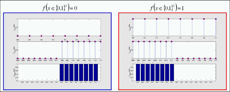
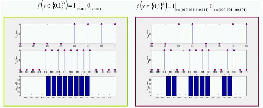
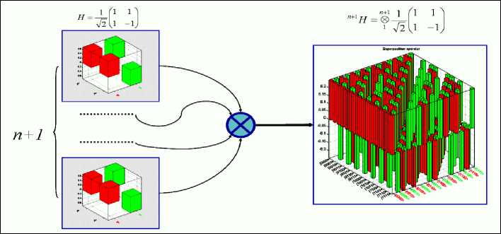
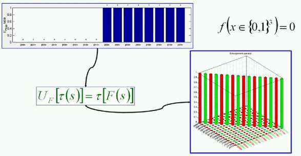
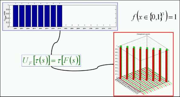
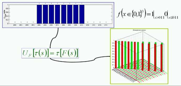
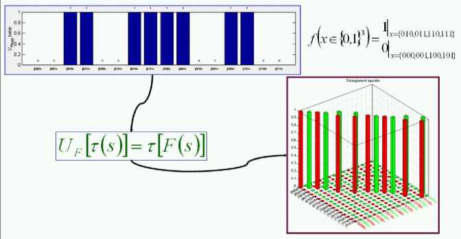
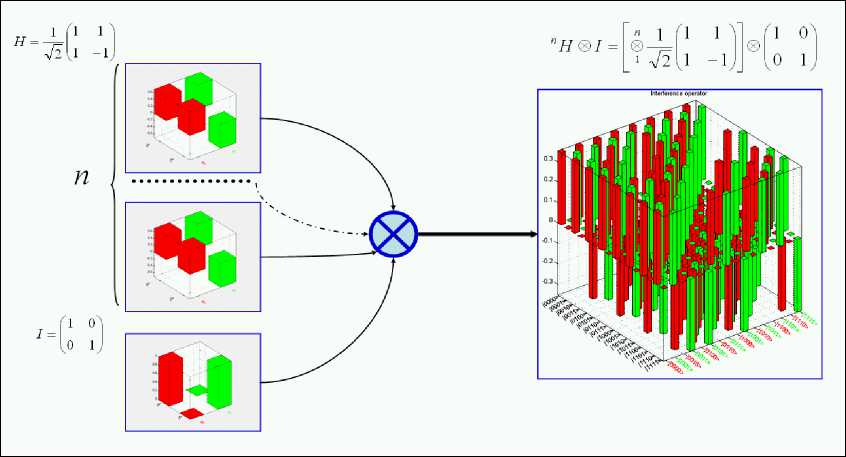
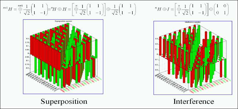
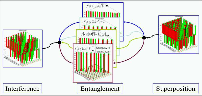
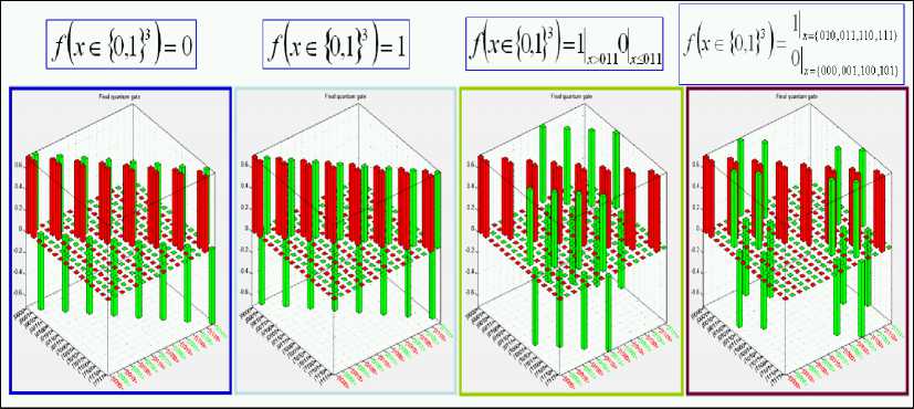
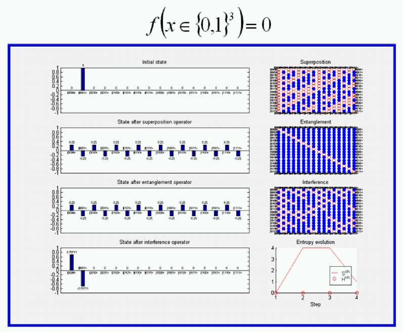
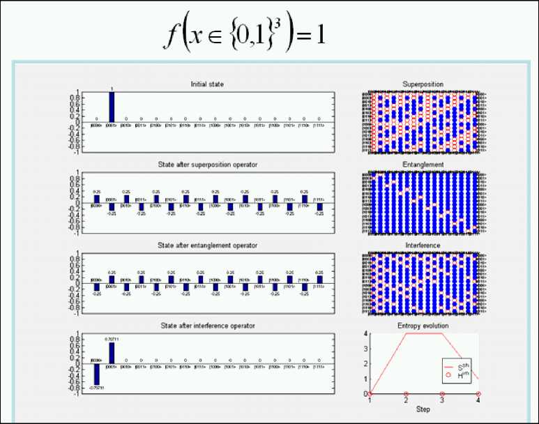
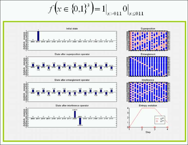
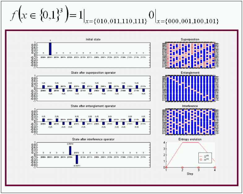
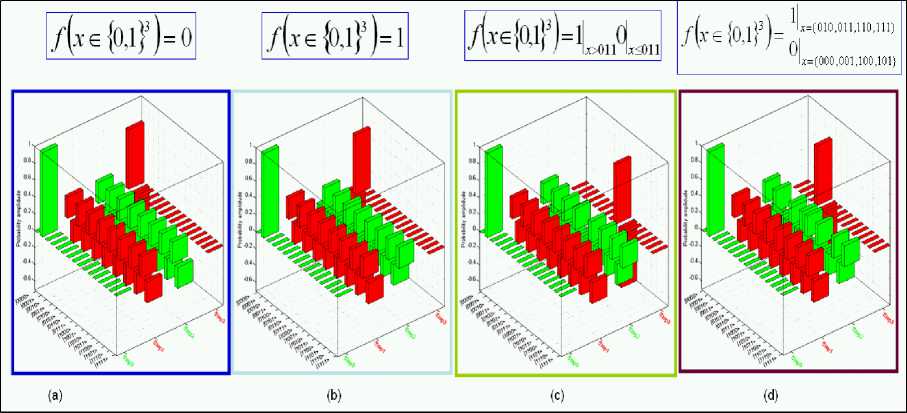
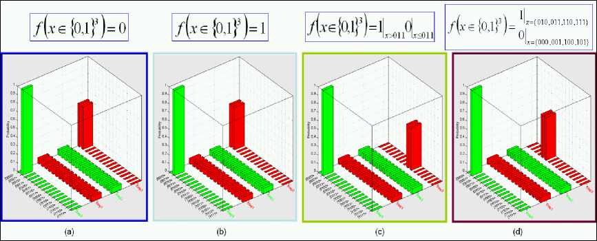
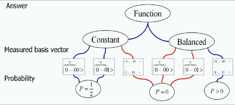
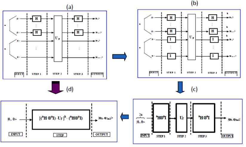
UF
|0..0>
|0..1>
… |1..1>
|0..0>
M0.. 0
0
… 0
|0..1>
0
M0.. 1
… 0
|1..1>
0
0
0 M1.. 1
where Mi= P1⊗..⊗Pn , Pk∈{I, C}, k = 1,..,n and and Mi = Mj ⇔ (j=i ∨ j=i⊕s).

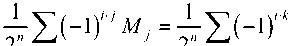
References Design information technology of quantum algorithm gates
- Ulyanov S.V., Ghisi F., Kurawaki I., Litvintseva L.V. Simulation of quantum algorithms on classical computer. - Note del Polo Ricerca, Università degli Studi di Milano (Polo Didattico e di Ricerca di Crema). - Milan, 1999. - Vol. 32.
- Ulyanov S.V., Kurawaki I., Yazenin A.V. et all. Information analysis of quantum gates for simulation of quantum algorithms on classical computers // Proceedings of Intern. Conf. on Quantum Communication, Measurements and Computing (QCM&C'2000). - Capri. Italy, 2000. Kluwer Acad. /Plenum Publ. - 2001. - Pр. 207-214.
- Ulyanov, S.V., Litvintseva V. L., Ulyanov, S.S. Quantum Information and Quantum Computational Intelligence: Design & Classical Simulation of Quantum Algorithm Gates. - Note del Polo Ricerca, Università degli Studi di Milano (Polo Didattico e di Ricerca di Crema). - Milan, 2003. - Vol. 80.
