Design of (FPID) controller for Automatic Voltage Regulator using Differential Evolution Algorithm

Published Online December 2019 in MECS DOI: 10.5815/ijmecs.2019.12.03

• I.    Introduction

  Fractional calculus in the last two centuries has been quite common research area in engineering study, although it has been recognized for about 300 years. The non-integer calculus begins with the 1965 [1].

Many methods were pro-positioned in the literature to design FOPID controller. You can classify these approaches into two groups: analytical methods and heuristic techniques. The parameters of the FOPID controller are tuned in the analytical framework by minimizing a nonlinear objective function based on the specific possibilities imposed by the developers.

To the extent numerous scholars have examined the heuristic procedures, rule-based strategies and transformative calculation based systems, Evolutionary calculations, for example, Genetic Algorithm (GA), Particle Swarm Optimization (PSO) and Electromagnetism, for example, algorithm (EM) are likewise used to plan FOPID controllers[2,3],in the literature provided the first research on the fractional order proportional-integral-derivative (FOPID) controller.

Unlike the classical PID[2] is proposing two extra parameters called π, μ for the fractional PID. Researchers have indicated that in terms of certain characteristics such as flexibility and stability, these two parameters reinforce the hand of customers.

Works on fractional controllers have been increasing day by day[4,5]. [6] proposed a solid FOPID controller for wind turbine generators. [7] suggested the design of the fractional order controller based on the technique of particle swarm optimization (PSO). Genetic algorithms have been used to design FOPID controllers by recasting the issue to a issue of optimization[8]. Different tuning techniques, such as altered method Ziegler-Nichols, have also been used by researchers to design a FOPID controller[9]. On the other side, there is a comprehensive debate about the efficiency of FOPID controllers intended by ABC Algorithm for tuning the PID controllers of the fractional order[10]. An important entity for the operation of the power system[11] is the automatic voltage regulator (AVR). Therefore, studying its modeling is essential to observe the conduct and efficiency of AVR. Because AVR is a complex system with a greater feature of order transfer, studying it is tedious. This article addressed and enforced the Biogeography-based Optimization (BBO) Model Reduction Scheme for this system. Differential Evolution(DE) has become increasingly common recently as a simple and impressive plot for global optimization over continuous spaces. In the current job, the FOPID controller system was screened using the DE algorithm and compared with others optimization methods,like(IWO,SCA).

• II.    AVR Modeling

The standards of AVR is to keep up the generator terminal voltage extents at the predetermined level. AVR framework comprises of four fundamental parts there are amplifer, exciter, generator and sensors. The numerical model can be considered linear and taking into account the time constant and neglecting the saturation or other nonlinearities. Fig.1 shows AVR model .

The AVR loop ensures that the terminal voltage in the power system is constant and stable. A voltage level sensor continually senses a terminal voltage. To compare with a DC reference signal in the comparator, it is rectified and smoothed. The error voltage from the comparator output is then amplified in an amplifier. Lastly, this signal is used to control the exciter winding of the generator field.

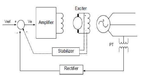
Fig.1. shows AVR model [12]

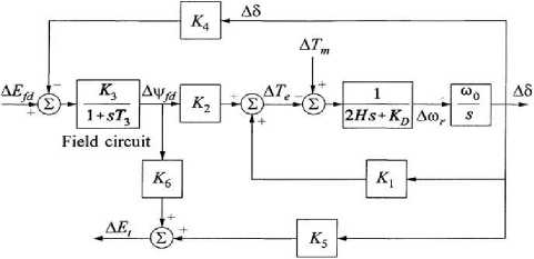
Fig.2. The Generator model[14]

D. Sensor model

The voltage is perceived through a possible electrical device and, in one kind, it's corrected through a bridge

rectifier. The device is modeled by a straightforward first

The AVR model consists of many elements, which are:-

order transfer function, constant can be[12,13] :-

Hs(s)

given by a gain and a time

K s

1 + T s s

A. Amplifier model

The excitation system is electronic equipment could also be a magnetic , rotating, or modern electronic . This equipment is described by a gain Ka and a time constant Ta therefore the transfer function is[12,13];-

G a ( s ) =

1 + TaS

Where K_a = [10, 400], T = [0.02, 0.1] sec

B. Exciter model

There is a spread of various excitation varieties. However, modern excitation systems use ac power supply through solid-state rectifiers like SCR. within the simplest type, the transfer function of a contemporary exciter is also described by time constant Te and a gain Ke. [12,13]:-

G e ( S ) =

K e

1 + T e s

Where K_e = [0.8, 1], T = [0.5, 1.0] sec.

C. Generator model

For AVR, we've thought of a simplified linearized model as shown in Fig.2 The transfer function of generator model will be expressed as[12,14]

Go, ( s ) =

2 HK з K 6 S ² + K з K 6 K d S + K 3 ® o ( K 1 K 6 - K ₂ K 5)

2 HK 3 S ¹ + (2 Н + K d T , ) S ² + ( K d + ® о Т з ) S + ® o ( K , - K 2 K 3 K 4 )

Where K_s = [0.1 1] and T = [0.01 0.7].

The open-loop transfer function of AVR, can be represented as [12,13]:-

G avr = G a * G e * G ol           (5)

Or can be written as:- a3S^ + aS + a0AVR = b5S5 + b4S4 + b3S3 + b^S2 + bS + b0   (6)

Where a0 = KaK®(K1K6 -K2K5)

a1 = KOKK6 KD

b5 = 2 Ht^t,b4 = 2 HT3t6 + 2 HT3t„ + 2 HTeTa + KDT3TeTa b 3 = 2 HT3 + 2 Нте + KDT3Te + 2 HTa + KDT3Ta + KDTeTa b2 = 2 Н + KDT3 + KDTe + ®oT3Te + KDTa + ®oT3Ta + ®oTeK 1Ta — ®oTeK2K 3K4Ta b1 = KD + ®oT3 + ®oK1Te — ®oTeK 2 K3 K4 + ®oTeK1 + ®oTaK 2 K3 K4 bo = ®o (K1 - K 2 K3 K4)

Refer to ref. [ 14 ], Where

^ 1 =1.591, K 2 =1.5, K 3 =0.333, K₄=1.8, K 5 =0.12, K₆ =0.3, 7 3 =1.91, Н =3, K_D=0, to₀=377.

The open-loop transfers function of AVR as:

____________________ 5.994 S ² + 825.2 ___________________

AVR = 0.573 S ⁵ + 7.176 S ⁴ + 51.06 S ³ + 451.1 S ² + 876.6 S + 260.8

Equation(7) shows the open-loop transfer function of AVR, it's necessary to managing closed loop to measure the dynamic transient response parameters (max overshot, settling and rise times, etc), so it should be insert the feedback activity sensor.

Fig.3 demonstrates how the AVR system sections are arranged as a closed loop. The sensor continually detects terminal voltage Vt(s) of the generator and compares it with the necessary reference voltage Vref(s). The amplifier amplifies the difference between the reference and the sensed terminal voltages (e.g. error voltage) and is used by the exciter to excite the generator.

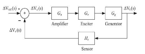
Fig.3. simplified AVR block diagram

Finally, the closed-loop transfer function (after connecting the sensor feedback element) is:-

V t ( s )        G AVR

V ref ( ^ )   1 + G AVR H s             (8)

V ( s )  _________________ 0.0599 s ³ + 5.994 s ² + 8.252 s + 825.2 _________________

V„ ( ss ) = 0.00573 s ⁶ + 0.644 s ⁵ + 7.686 s ⁴ + 55.571 s ³ + 465.86 s ² + 879.208 s + 1086 (9)

• III.    AVR model Reduction

Model order reduction (MOR) primarily retains the foremost necessary properties throughout modelling whereas rejecting unwanted or slighter parameters. The dimension massive of huge of enormous} scale system is thus large that standard techniques of modelling, simulation, control, analysis and computation fail to supply possible solutions with affordable machine efforts. Thus, the reduction of dimension of higher-order system is a straightforward tool in order that the higher than mentioned needs will be met with lesser complexness and value as a result of complexness of a system will increase with system order. In literature, mathematical approaches/algorithms to cut back the order of a higher-order system diagrammatic mathematically however applications area unit least [15,16]. The transfer function of AVR as apper in equation(9) is sixth order , so we've tried to approximate it to second order. Ref[17],shows several ways to scale back the order of AVR, classical(Truncation, Routh alpha beta approximation, Time moment matching, Pade approximation) and a computer power-assisted ways, like(PSO), big bang big Crunch(BBC),Genetic Algorithm(GA).

BBO algorithm for reducing order of AVR

It presents a biogeography-based optimization (BBO) rule to cut back model of AVR. Biogeography is that the science of the geographical distribution of biological species. The models of biological science make a case for however a organisms arises, immigrate from an surroundings to a different and gets eliminated. The planned rule has some common options with alternative population-based algorithms. Like GA & PSO, BBO additionally shares information amongst the solutions; however BBO doesn't involve in reproduction like GA. The BBO rule is principally supported two steps: migration and mutation. The BBO has some smart options in aiming to the worldwide minimum compared to alternative biological process algorithms [18].

There is necessary reason to think about BBO as a separate optimization rule, which is as a result of the biological science roots of BBO open up several avenues for extensions and modifications that might rather be unobtainable to the scientist. The BBO rule may be a easy, strong and novel international optimization methodology. BBO has sensible optimization performance because of its migration and mutation operators [19]. The BBO rule is especially supported two steps: migration and mutation.

Migration

In BBO formula, a population is chosen as an answer. This answer will represent as a vector of real number that every real number could be a SIV(suitability index variable) in BBO formula . The fitness of every answer will be calculated with its objective operate. This fitness is that the same HIS(habitat quality index) in BBO formula. In BBO answers with high HSI represents a decent answer and answer with low HSI represents a foul solution.

Mutation

Sudden changes in climate of one environs or alternative incidents can cause the fast changes in HSI of that environs . In BBO algorithmic program, this case are often model within the sort of fast changes in price of SIV. For a lot of details, see Ref[20 ]. The method of the BBO algorithmic program for reducing model order of AVR was enforced in MATLAB software package. For this case study, generation count limit=200, population size=50,     proplem     dimension=5,     mutation probability=0.06, number of elites=2, after exploitation improvement program, the reduced transfer perform of AVR is:-

_     0.0003217 s + 2.401

Gr = -------5----------------- r 1.277 s2 + 2.386 s + 3.171

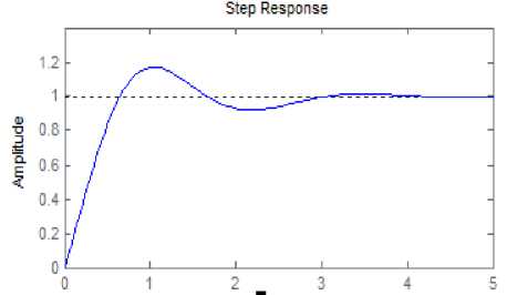
There are no large differences between original and reduced order systems, where both have the same overshot(Mp%),settling time(Ts) , rise time(Tr),peak time(Tp) and steady-state error(Ess),Fig.4 shows transient response of original and reduced order systems. For simplicity in design and analysis, equation(10) can be used instead of equation(9).

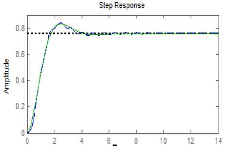
Fig.4. shows step response of original and reduced order system

As seen from Fig. 4 the transient specifications are almost identical, where the blue is original system and the green reduced system. The transient data parameters are calculated by using Matlab package. Table 1. Shows comparison parameters between original and reduced system.

Table 1. Transient response parameters comparison

System	Mp%	Ts(sec)	Tp(sec)	Tr(sec)	Ess
Original	10.9	4.5	2.42	1.03	0
Reduced	9.9	3.76	2.46	1.17	0.757

• IV.    FPID Controller

The FOPID controller comprises of two extra parameters called n and ц which define integration and differentiation orders unlike the conventional PID. These two parameters provide the controller with flexibility and durability. Four distinct objective features are used to examine the controller's efficiency: ISE, ITSE, IAE and ITAE.Thus, in equations.(11)-(14) the objective features used in this research phase are provided:

to

ISE = J e 2( t) d (t)(11)

0 to

ITSE = J t .e 2( t) d (t)

0 to

IAE = Je (t)dt.(13)

ITAE = j t . e ( t ) dt .

The continuous transfer function of FOPID is also obtained through Laplace transform as:

C ( 5 ) = Kp + Ki + Kds ^ц s ^л

Where Kp is proportional constant ,Ki is integral constant, and Kd is derivative constant while fractional powers (X and ц) of the integral and derivative parts respectively add to the better flexibility of Fractional PID controller.

Firstly, the tuning is done to obtain the parameters of PID controller Kp, Ki and Kd by Ziegler-Nichols(Z-N) ,by using closed-loop control system with Kp only and change it until reach sustained oscillation, after that read the critical gain(Kcr) and ultimate frequency(Pcr),return to (Z-N) table and calculate, Kp=4.22,Ki=5.31, and Kd=0.84.

Fig.5 shows the transient response of Gr with Z-N PID controller,,Mp=17.1%,Ts=2.84sec,Tr=0.493sec,Tp=1.03s ec and Ess=0. Different tuning methods have been used to tune fractional order PID controller, but in this paper, it is used Differential Evolution (DE) algorithm.

Fg.5. shows step response of reduced order system with PID controller

DE-based tuning FPID controller

DE algorithm is a stochastic method of optimization that minimizes an objective function that, while incorporating constraints, can model the objectives of the problem. DE is a fairly fresh method for optimization. It is very simple to implement, needs little or no parameter tuning and has been implemented effectively in many issues domain The algorithm primarily has three benefits; discovering the real global minimum irrespective of original parameter values, quick convergence, and using a few control parameters[21]; Being simple, quick, easy to use, easy to adapt for integer and discrete optimization, quite efficient in the optimization of nonlinear constraints including penalty functions and useful for optimizing multi-modal search spaces are the other important features of DE [22,23].

The DE algorithm is a population-based algorithm that uses comparable operators like genetic algorithms; crossover, mutation, and choice. In building better alternatives, the primary distinction is that genetic algorithms depend on crossover while DE focuses on mutation operation. This primary procedure is based on variations in population between randomly sampled pairs of alternatives. The rule uses mutation operation as a groundwork mechanism and choice operation to direct the search toward the possible regions within the search space. The DE rule additionally uses a non-uniform crossover that may take DE vector parameters from one parent a lot of typically than it will from others. By using the elements of the present population members to construct trial vectors, the recombination (crossover) operator expeditiously shuffles data regarding successful combinations, enabling the look for a much better answer area. the most steps of the de rule ar, initialization, Evaluation, Repeat, Mutation, Recombination, Evaluation ,Selection, till (termination criteria are met).The block-diagram of DE is shown in Fig.6

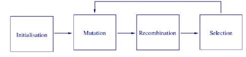
Fig.6. shows the block-diagram of DE procedures

It should be observed that the unified parameter settings are as follows, except for unique instructions. Population size pop size (NP)= 10, reduced bound scaling factor F1=0.2, upper bound F2=0.8, crossover likelihood Cr=0.2. The technique of mutation utilizes "DE / Rand/1" and 150 iterations maximum. If the ideal theoretical solution is discovered, the program will end. Equ(11-14) was used as the four performance index. The lower bound of decision variables[ 00000]and the upper bound of decision variables[ 10 10 1.5 10 1.5].Matlab package can be used to execute DE procedures of fig.6.untill reach the maximum iterations. Table 2. indicates the FPID controller values depending on the performance index.

Table 2. Parameters values of FPID controller with different performance index(P.I) using DE algorithm

There are several strategies obtainable in literature to approximate the fractional order. a number of the wide used frequency domain approaches area unit Carlson's methodology, Matsuda's methodology, Oustaloup's methodology and Chareff 's methodology, during this paper the crone approximation methodology given in [24] is employed. The designed FOPID controller is approximated by oustaloup filter. The fractional derivative and integrals of FOPID controller have been approximated by N=5 and filter frequency [Wl,Wh] =[0.001,1000].The Mat lab program is:- clear clc;

nn=[0.0003217 2.401];

dd=[1.277 2.386 3.171];

g=tf(nn,dd);

C=fracpid(Kp,Ki, λ ,Kd, µ ); f=series(g,C);

sysc=feedback(f,1);

syscint=oustapp(sysc,0.001,1000,5);

t=0:0.01:5;

step(syscint,g,t) s=stepinfo(syscint)

Table 3. shows transient parameters with different ( P.I), after executing the matlab program.

Table 3.Transient parameters values of FPID controller with different performance index using DE algorithm

P.I	Ts(sec)	Tr(sec)	Mp%	Ess
ISE	22.9325	3.9697e-04	0.9898	0
ITSE	1.0527	0.2594	0.0495	0
IAE	0.9345	0.3010	0.0187	0
ITAE	0.4976	0.2884	0.0922	0

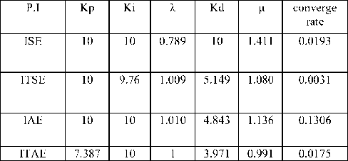
For comparison DE algorithm with other optimization techniques (IWO),(SCA), and because the paper size limitation, all these techniques are not considered in detail, so that ,for (IWO) refer to Ref[25],and let the parameters of algorithm are:-

Varmin=[0 0 0 0 0],Varmax=[ 10 10 1.5 10 1.5], maximum number of iterations=150, initial population size=2,maximum population size=10,minimum number of seeds=0,maximum number of seeds=5, variance reduction exponent=2,initial value of standard deviation=0.5 and final value of standard deviation=0.001.Table 4. indicates the FPID controller values depending on the performance index.

Table 4. Parameters values of FPID controller with different performance index using IWO algorithm

P.I	Kp	Ki	λ	Kd	µ	converge rate
ISE	10	10	0.789	10	1.412	0.0193
ITSE	10	10	1.001	6.477	1.020	0.0032
IAE	9.623	10	1.014	4.480	1.126	0.1308
ITAE	5.136	8.66	1	3.336	0.875	0.0427

Table 5. shows transient parameters with different performance index, after executing the matlab program

Table 5. Transient parameters values of FPID controller with different performance index using IWO algorithm

Performance index	Ts(sec)	Tr(sec)	Mp%	Ess
ISE	6.7437	2.0701e-07	1.0031	0
ITSE	1.5706	0.2058	0	0
IAE	0.8068	0.3043	0.0026	0
ITAE	0.8176	0.3259	2.1734	0

Again ,when compared with(SCA) algorithm, refer to Ref[26], and let the parameters of algorithm are:-

Table 6. Parameters values of FPID controller with different performance index using SCA algorithm

P.I	Kp	Ki	λ	Kd	µ	converge rate
ISE	10	10	0.845	10	1.421	0.019606
ITSE	9.620	10	1.045	7.776	0.827	0.004288
IAE	7.698	9.88	1	4.535	0.960	0.13915
ITAE	9.402	9.78	1.003	4.358	0.882	0.089436

Table 7. shows transient parameters with different performance index, after executing the matlab program

Table 7. Transient parameters values of FPID controller with different performance index using SCA algorithm

Performance index	Ts(sec)	Tr(sec)	Mp%	Ess
ISE	17.5373	2.5549e-04	1.9174	0
ITSE	1.8569	0.1835	1.8087	0
IAE	0.4577	0.2582	0.1638	0
ITAE	1.5877	0.2761	1.9187	0

• V.    Results Comparison And Discussion

  As seen from Tables 2.,4.,6.,the least values of convergence rate appears with (ITSE) performance index, DE algorithm gives optimum minimization with rate(0.0031) .Fig.7 shows the transient response of all optimization algorithms (DE,IWO,SCA) and Z-N method.

When compared transient parameters (Ts, Tr, Mp%) values of FPID controllers, The DE method appears very speed response because it gives minimum(Ts),While the Mp% approaches to zero. The ZN-PID appears bad response, when compared with DE,IWO and SCA,because gives sluggish response with maximum Mp% and needs more tuning. Table 8. Shows the comparison between all optimization methods for designing PID controller.

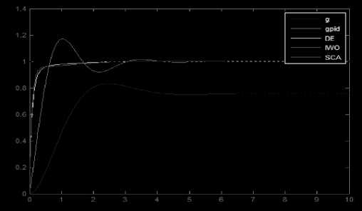
Fig.7. shows transient response of all optimizations methods

Table 8. Comparison between all optimizations methods for PID controller

Optimization method	Ts(sec)	Tr(sec)	Mp%	Ess
ZN-PID	2.84	0.493	17.1	0
IWO-PID	1.5706	0.2058	0	0
SCA-PID	1.8569	0.1835	1.8087	0
DE-PID	1.0527	0.2594	0.0495	0

• VI.    Conclusions

In this article an AVR scheme with automatic PID controller was optimally tuned using Differential Evolution (DE) algorithm and contrasted with (IWO, SCA) algorithms for proportional, integral and derivative gains. Different time domain requirements are regarded for this issue, such as maximum peak overshoot, settling time, rise time, and so on. In an attempt to study the impact of the performance index on the requirements of the time domain, the fitness function is provided distinct performances. Software simulation of the system with different fitness function revealed that the time domain specification of the DE algorithm gives the best values, especially the response speed and this situation is very important for AVR ,also there is no vibration or chattering at the steady state part ,generally (ITSE) performance index shows better compared with others indexes(ISE,IAE,,ITAE).In addition, the proposed study depicts that, the performance of DE is better than classical tuning of PID structure, using the famous Z-N procedures. This work can be expended to take nonlinear AVR model in future work, also using some comparison with intelligent (fuzzy,Neural Network) controllers.

Acknowledgment

The authors would like to thank Mustansiriyah University ( Baghdad – Iraq for its support in the present work.