Designing of a cavitation heat generator for heating water with a capacity of 10 kW

Бюллетень науки и практики / Bulletin of Science and Practice

UDC 662.995                                        

The traditional heating and heating method consumes a lot of fuel and costs a lot. Facing the current situation of energy shortage and serious pollution to the environment caused by fuel combustion, it is urgent to develop a new heating and heating method. As an environmentally friendly and cost-effective, alternative sources of thermal energy, it is proposed to use pulsed physical and chemical effects in a liquid, which lead to its heating. An effective method of multifactorial influence on a liquid is cavitation, which leads to a change in the physicochemical characteristics of the liquid, its activation and heating. The liquid cavitation generator uses electricity as the power, liquid as the medium, and cavitation effect as the core technology. It uses the cavitation phenomenon to convert liquid kinetic energy into heat energy, which changes the traditional heating method. Zero emission, no pollution, good environmental protection, greatly reduced heating costs.

In 1897, S. W. Barnaby and C. A. Parsons [1, 2] put forward the concept of “cavitation” on the basis of experimental research and believed that the high-speed relative motion between solid and liquid might lead to cavitation.

Lord Rayleigh [3] was the first to systematically analyze cavitation and cavitation movement. In 1917, he put forward a more systematic cavitation theory and established an idealized spherical cavitation movement equation.

Yasui [4], a Japanese scholar, believes that evaporation and condensation in the medium also have a greater impact on the cavitation movement.

In 2021, Zhang [5] et al. of Jiangsu University in China used a new type of cavitating cannonless forming technology to simulate the whole movement process of laser induced cavitation from birth to collapse, and studied and analyzed the cavitation collapse shock wave and high-speed micro jet. The improvement of the bubble motion equation enriches people's understanding of the process of bubble growth, development, collapse, and promotes the development of bubble dynamics.

Wu [6] et al. of Peking University established a three-dimensional fully coupled model considering the fluid disturbance on both sides of the thin-walled plate to study the interaction between bubbles and thin-walled plates. This model can describe the hydrodynamic balance on both sides of the submerged plate, The vibration characteristics and elastic-plastic deformation of the flat plate under the violent load of bubbles are analyzed. Neppiras [7] et al. show that the bubble will produce subharmonics in the process of vibration.

Deng [8] et al. established a model of non spherical bubbles in compressible liquid under the coupling effect of ultrasound and electrostatic field. After research, they found that under the combined effect of ultrasound radiation and electrical stress, the non-spherical bubbles could not oscillate stably in the liquid, and the bubbles would inevitably break in several cycles.

Dittakavi [9] studied sheet cavitation and cloud cavitation in Venturi tube by using large eddy simulation and found that the high frequency noise increases correspondingly when cavitation occurs.

Li [10, 11] et al. of Huazhong University of Science and Technology found that the influence of the inlet discontinuity on the pressure amplitude and peak value is relatively complicated, but both of them have a positive effect on the mass loss caused by cavitation. Positive effect; the amplitude and peak value of the vibration are maximum when the exit angle is 0°С.

In 2012, Zhang Fenghua’s team [12] of Hunan University of Technology put forward a new type of choking cavitation device based on a series of gas-liquid two-phase flow choking cavitation phenomena and simulated sewage treatment. This kind of choked cavitation device can form a large cavitation area, and the void in the cavitation area.

In 2017, P. G. Suryawanshi [13] and N. B. Suryawanshi [14] found that the vortex secondary can produce larger cavitation area and higher cavitation efficiency through experimental comparison with orifice cavitation generator.

Due to the complexity, subjectivity, multiphase and randomness of the cavitation process, and because the cavitation process is affected by many factors at the same time, the theoretical research on cavitation still needs to be further improved and studied. This article establishes a threedimensional model of the design circuit of a water heating cavitation device and simulates it in Hysys software. The relationship between temperature, pressure and flow rate of cavitation generator in pulsed heating water circulation unit is studied by using control variables. The dependence of pressure and temperature difference on flow rate was studied. The dependence of pressure and temperature difference on the thermal power of the cavitation device was studied. The dependence of pressure and temperature differences on pipeline diameter was investigated.

Unit Description for Simulation

During the research phase, a pulsating loop model was developed. Figure 1 shows a threedimensional model for designing the circuit of a water heated cavitation generator device.

Before starting work, all circuits of the laboratory installation are filled with a working fluid (the water at normal temperature and pressure at 25 ℃ and 100KPa). In the 3D model design cycle circuit diagram, when the circulating pump is turned on, it takes water from the expansion tank and pumps it to two branches. Branch route 1: Water is heated through a cavitation generator and then flows back to the expansion tank through the main route. Branch route 2: Water flows through the shock assembly and then enters the main road back to the expansion tank.

Figure 2 shows the 3.25 kW cavitation model. Cavitator for heat release in liquid has cylindrical housing 1 with Venturi tube 2 located coaxially inside its Venturi tube holds insert 4 Screw feeder 3 is mounted before insert 4 on Venturi tube 2 on side of incoming flow for rotation about Venturi tube. Insert 4 extends beyond Venturi tube 2 on side of scope of flow Outer surface of insert 4 is provided with longitudinal slots 5 open on side of screw feeder 3 and brought in communication with outlet surface of insert 4 on opposite side by means of holes 6.

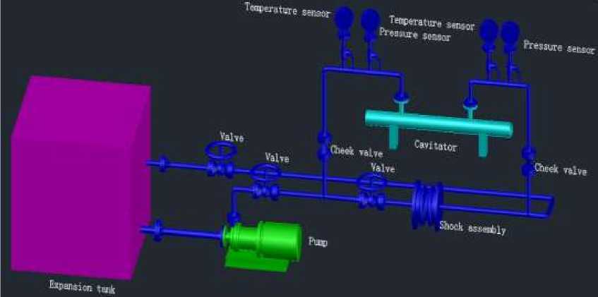
Figure 1. A 3-dimensional diagram of Water heating cavitation generator circuit

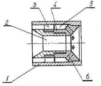
Figure 2. Scheme of cavitator

As a new type of heat source device, its working principle is that when the liquid flows through the cavitation generator under the effect of kinetic energy, the liquid flow speed will sharply increase in the basin where the flow section suddenly drops, resulting in a sudden drop in pressure. When the pressure is lower than the saturated Vapor pressure, a large number of tiny bubbles will be generated in the liquid. The bubbles will quickly break and friction through the impact, releasing a strong shock wave, and at the same time, high temperature and high pressure will also be generated, the kinetic energy is converted into thermal energy, which causes the liquid to heat up. Liquid cavitation generator, powered by electricity and liquid as medium, with cavitation effect as the core technology, utilizes cavitation phenomenon to convert liquid kinetic energy into heat energy, changing the traditional heating method. It integrates heat generation and heat medium transportation and has good environmental protection.

Expansion water tank: In this circulating circuit, it can accommodate the expansion of system water and play a constant pressure role in supplementing the system with water. The material of the water tank is plastic, and there is a baffle in the water tank. The setting of the baffle can reduce the flow speed of tap water in the water tank, increase the residence time in the water tank, and effectively reduce bubbles in the water tank, which is conducive to the stability of the water flow state in the pipeline.

Pump: Conveys fluid water and pressurizes the water, transferring the mechanical energy or other external energy of the prime mover to the water supply, enhancing the energy of the water.

Valve: used to regulate and throttle the flow of water.

Check valve: prevents water backflow, reverse rotation of pump and drive motor, and discharge of container medium.

Shock assembly: At the beginning, the shock assembly is closed, and all working fluid flows through the cavitator and returns to the expansion tank after being heated. When the working fluid flowing through the cavitation device reaches a certain pressure, the shock assembly opens to prevent vibration caused by excessive pressure in the cavitation device. The frequency of the shock assembly switch is 2.5 Hz, opening for 0.3 seconds and then closing for 0.1 seconds, in a cyclic manner. The shock assembly can provide periodic pulses, which can increase the Reynolds number, thus improving the heating efficiency of the cavitation generator.

Temperature sensor: measures the temperature of the working fluid water before and after the cavitation device. Pressure sensor: measures the pressure of the working fluid before and after the cavitation device.

In order to clearly identify the interrelationships between temperature, pressure, and flow rate of the cavitation generator. We simulated the instantaneous changes in pressure after cavitation generator and temperature difference before and after cavitation generator over time under different flow rates, pipe diameters, and power conditions. We studied the variation of temperature after cavitation generator and temperature difference before and after cavitation generator with flow rate under a certain power. We studied the changes in temperature after the cavitation generator and the temperature difference before and after the cavitation generator with power under a certain flow rate. Figure 3 is a Hysys simulation flowchart of a 10kW cavitation generator. Figure 4 is a Hysys simulation flowchart of two parallel 5 kW cavitation generators. Figure 5 is a Hysys simulation flowchart of three parallel 3.25 kW cavitation generators.

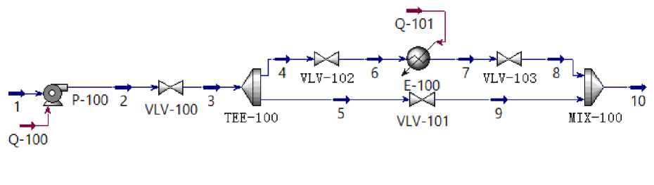
Figure 3. Hysys simulation flowchart for a 10kW cavitation generator

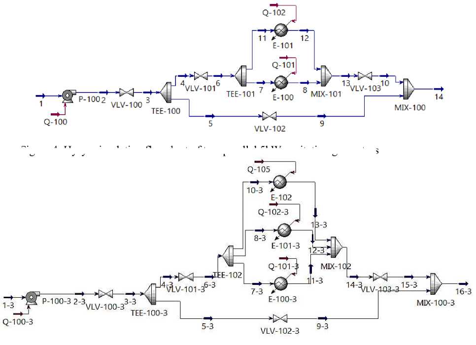
Figure 5. Hysys simulation flowchart of three parallel 3.25 kW cavitation generators

Figure 4. Hysys simulation flowchart of two parallel 5kW cavitation generators

Results and discussion

The simulation results are shown in Table 1-5. The name label corresponds to the name in the simulation diagram in the previous chapter.

Table 1

STATIC SIMULATION RESULTS WHEN TOTAL G=0.42M3/H, POWER=10 KW, D=100MM

Simulated data table when the shock assembly is closed

Name	1	2	3	4	5
Temperature, °C	25	25.0197	25.0197	25.0197	25.0197
Pressure, KPa	100	300	300	300	300
Molar Flow, kgmole/h	23.31378	23.31378	23.31378	23.31378	0
Mass Flow, kg/h	420	420	420	420	0
Liquid Volume Flow, m3/h	0.420848	0.420848	0.420848	0.420848	0
Name	6	7	8	9	10
Temperature, C	25.0197	45.51297	45.55467	25.06398	45.55467
Pressure, KPa	300	300	100	100	100
Molar Flow, kgmole/h	23.31378	23.31378	23.31378	0	23.31378
Mass Flow, kg/h	420	420	420	0	420
Liquid Volume Flow, m3/h	0.420848	0.420848	0.420848	0	0.420848
Simulated data table when the shock assembly is open
Name	1	2	3	4	5
Temperature, C	25	25.0197	25.0197	25.0197	25.0197
Pressure, KPa	100	300	300	300	300

Бюллетень науки и практики / Bulletin of Science and Practice Т. 9. №9. 2023 Simulated data table when the shock assembly is open Name 1 2 3 4 5 Molar Flow, kgmole/h 23.31378 23.31378    23.31378 9.991618 13.32216 Mass Flow, kg/h 420 420 420 180 240 Liquid Volume Flow, m3/h 0.420848 0.420848    0.420848 0.180363 0.240484 Name 6 7 8 9 10 Temperature, °C 25.0197 72.79751     72.83614 25.06398 45.55467 Pressure, KPa 300 300 100 100 100 Molar Flow, kgmole/h 9.991618 9.991618    9.991618 13.32216 23.31378 Mass Flow, kg/h 180 180 180 240 420 Liquid Volume Flow, m3/h 0.180363 0.180363    0.180363 0.240484 0.420848 STATIC SIMULATION RESULTS WHEN TOTAL G=0.42M3/H, POWER= 10 KW, D= Table 2 150 MM Simulated data table when the shock assembly is closed Name 1 2 3 4 5 Temperature, °) 25 25.0197 25.0197 25.0197 25.0197 Pressure, KPa 100 300 300 300 300 Molar Flow, kgmole/h 23.31378 23.31378    23.31378 23.31378 0 Mass Flow, kg/h 420 420 420 420 0 Liquid Volume Flow, m3/h 0.420848 0.420848    0.420848 0.420848 0 Name 6 7 8 9 10 Temperature, C 25.0197 45.51297    45.55467 25.06398 45.55467 Pressure, KPa 300 300 100 100 100 Molar Flow, kgmole/h 23.31378 23.31378    23.31378 0 23.31378 Mass Flow, kg/h 420 420 420 0 420 Liquid Volume Flow, m3/h 0.420848 0.420848    0.420848 0 0.420848 Simulated data table when the shock assembly is open Name 1 2 3 4 5 Temperature, C 25 25.0197 25.0197 25.0197 25.0197 Pressure, KPa 100 300 300 300 300 Molar Flow, kgmole/h 23.31378 23.31378    23.31378 9.991618 13.32216 Mass Flow, kg/h 420 420 420 180 240 Liquid Volume Flow, m3/h 0.420848 0.420848    0.420848 0.180363 0.240484 Name 6 7 8 9 10 Temperature, C 25.0197 72.79751     72.83614 25.06398 45.55467 Pressure, KPa 300 300 100 100 100 Molar Flow, kgmole/h 9.991618 9.991618    9.991618 13.32216 23.31378 Mass Flow, kg/h 180 180 180 240 420 Liquid Volume Flow, m3/h 0.180363 0.180363    0.180363 0.240484 0.420848 STATIC SIMULATION RESULTS WHEN TOTAL G=0.56M3/H, POWER= 10 KW, D= Table 3 100 MM Simulated data table when the shock assembly is closed Name 1 2 3 4 5 Temperature, C 25 25.0197 25.0197 25.0197 25.0197 Pressure, KPa 100 300 300 300 300 Molar Flow, kgmole/h 31.08503 31.08503    31.08503 31.08503 0

Бюллетень науки и практики / Bulletin of Science and Practice Т. 9. №9. 2023 Simulated data table when the shock assembly is closed Name 1 2 3 4 5 Mass Flow, kg/h 560 560 560 560 0 Liquid Volume Flow, m3/h 0.56113 0.56113 0.56113 0.56113 0 Name 6 7 8 9 10 Temperature, °C 25.0197 40.39031     40.43262 25.06398 40.43262 Pressure, KPa 300 300 100 100 100 Molar Flow, kgmole/h 31.08503 31.08503    31.08503 0 31.08503 Mass Flow, kg/h 560 560 560 0 560 Liquid Volume Flow, m3/h 0.56113 0.56113 0.56113 0 0.56113 Simulated data table when the shock assembly is open Name 1 2 3 4 5 Temperature, C 25 25.0197 25.0197 25.0197 25.0197 Pressure, KPa 100 300 300 300 300 Molar Flow, kgmole/h 31.08503 31.08503    31.08503 13.32216 17.76288 Mass Flow, kg/h 560 560 560 240 320 Liquid Volume Flow, m3/h 0.56113 0.56113 0.56113 0.240484 0.320646 Name 6 7 8 9 10 Temperature, C 25.0197 60.87008    60.91003 25.06398 40.43262 Pressure, KPa 300 300 100 100 100 Molar Flow, kgmole/h 13.32216 13.32216 13.32216 17.76288 31.08503 Mass Flow, kg/h 240 240 240 320 560 Liquid Volume Flow, m3/h 0.240484 0.240484    0.240484 0.320646 0.56113

Table 4

STATIC SIMULATION RESULTS WHEN TOTAL G=0.42M³/H, TWO PARALLEL POWER=5×2KW, D=100MM

Simulated data table when the shock assembly is closed

Name	1	2	3	4	5
Temperature, C	25	25.0197	25.0197	25.0197	25.0197
Pressure, KPa	100	300	300	300	300
Molar Flow, kgmole/h	23.31378	23.31378	23.31378	23.31378	0
Mass Flow, kg/h	420	420	420	420	0
Liquid Volume Flow, m3/h	0.420848	0.420848	0.420848	0.420848	0
Name	6	7	8	9	10
Temperature, C	25.0197	25.0197	45.51183	25.06398	45.55353
Pressure, KPa	300	300	300	100	100
Molar Flow, kgmole/h	300	11.65689	11.65689	0	23.31378
Mass Flow, kg/h	300	210	210	0	420
Liquid Volume Flow, m3/h	300	0.210424	0.210424	0	0.420848
Name	11	12	13	14
Temperature, C	25.0197	45.51183	45.51183	45.55353
Pressure, KPa	300	300	300	100
Molar Flow, kgmole/h	11.65689	11.65689	23.31378	23.31378
Mass Flow, kg/h	210	210	420	420
Liquid Volume Flow, m3/h	0.210424	0.210424	0.420848	0.420848

Simulated data table when the shock assembly is open
Name	1	2	3	4	5
Temperature, °C	25	25.0197	25.0197	25.0197	25.0197
Pressure, KPa	100	300	300	300	300
Molar Flow, kgmole/h	23.31378	23.31378	23.31378	9.991618	13.32216
Mass Flow, kg/h	420	420	420	180	240
Liquid Volume Flow, m3/h	0.420848	0.420848	0.420848	0.180363	0.240484
Name	6	7	8	9	10
Temperature, C	25.0197	25.0197	72.79486	25.06398	72.83349
Pressure, KPa	300	300	300	100	100
Molar Flow, kgmole/h	9.991618	4.995809	4.995809	13.32216	9.991618
Mass Flow, kg/h	180	90	90	240	180
Liquid Volume Flow, m3/h	0.180363	0.090182	0.090182	0.240484	0.180363
Name	11	12	13	14
Temperature, C	25.0197	72.79486	72.79486	45.55353
Pressure, KPa	300	300	300	100
Molar Flow, kgmole/h	4.995809	4.995809	9.991618	23.31378
Mass Flow, kg/h	90	90	180	420
Liquid Volume Flow, m3/h	0.090182	0.090182	0.180363	0.420848

STATIC SIMULATION RESULTS WHEN TOTAL G=0.42M3/H, THREE PARALLE POWER=3.25x3KW, D=100 MM						Table 5
Simulated data table when the shock assembly is closed
Name	1	2	3	4	5	6
Temperature, C	25	25.0197	25.0197	25.0197	25.0197	25.0197
Pressure, KPa	100	300	300	300	300	300
Molar Flow, kgmole/h	23.31378	23.31378	23.31378	23.31378	0	23.31378
Mass Flow, kg/h	420	420	420	420	0	420
Liquid Volume Flow, m3/h	0.420848	0.420848	0.420848	0.420848	0	0.420848
Name	7	8	9	10	11	12
Temperature, C	25.0197	25.0197	25.06398	25.0197	44.99922	55.75159
Pressure, KPa	300	300	100	300	300	300
Molar Flow, kgmole/h	7.771258	7.771258	0	7.771258	7.771258	7.771258
Mass Flow, kg/h	140	140	0	140	140	140
Liquid Volume Flow, m3/h	0.140283	0.140283	0	0.140283	0.140283	0.140283
Name	13	14	15	16
Temperature, C	44.99922	48.58427	48.62562	48.62562
Pressure, KPa	300	300	100	100
Molar Flow, kgmole/h	7.771258	23.31378	23.31378	23.31378
Mass Flow, kg/h	140	420	420	420
Liquid Volume Flow, m3/h	0.140283	0.420848	0.420848	0.420848
Simulated data table when the shock assembly is open
Name	1	2	3	4	5	6
Temperature, C	25	25.0197	25.0197	25.0197	25.0197	25.0197
Pressure, KPa	100	300	300	300	300	300
Molar Flow, kgmole/h	23.31378	23.31378	23.31378	9.991618	13.32216	9.991618
Mass Flow, kg/h	420	420	420	180	240	180
Liquid Volume Flow, m3/h	0.420848	0.420848	0.420848	0.180363	0.240484	0.180363
Тип лицензии CC: Attribution 4.0 International (CC BY 4.0)						195

Бюллетень науки и практики / Bulletin of Science and Practice Т. 9. №9. 2023 Simulated data table when the shock assembly is open Name 7 8 9 10 11 12 Temperature, °C 25.0197 25.0197 25.06398 25.0197 71.60204 96.57711 Pressure, KPa 300 300 100 300 300 300 Molar Flow, kgmole/h 3.330539 3.330539 13.32216 3.330539 3.330539 3.330539 Mass Flow, kg/h 60 60 240 60 60 60 Liquid Volume Flow, m3/h 6.01E-02 6.01E-02 0.240484 6.01E-02 6.01E-02 6.01E-02 Name 13 14 15 16 Temperature, C 71.60204 79.94044 79.97828 48.62562 Pressure, KPa 300 300 100 100 Molar Flow, kgmole/h 3.330539 9.991618 9.991618 23.31378 Mass Flow, kg/h 60 180 180 420 Liquid Volume Flow, m3/h 6.01E-02 0.180363 0.180363 0.420848

According to the experimental data results given in Tables 1-5, the temperature difference and pressure at the inlet and outlet of the cavitation system are plotted over time (Figure 6-12).

Pressure calculation formula : P = P_ST atic + P dynamic = P static + ¹P^²

• 1.    Open: P = 300 + 1 x 103кд/т3 x 53. 52 = 1730KPa

• 2.    Open: P = 300 + 1 x 10³кд/т³ x 23.8² = 582KPa

• 3.    Open: P = 300 + 1 x 10³кд/т³ x 71.33² = 2844KPa

Close: P = 300 +¹ x 10³кд/т³ x 22.9² = 562KPa

Close: P = 300 + 1 x 10³кд/т³ x 10.19² = 352KPa

Close: P = 300 + 1 x 10³кд/т³ x 30.57² = 767KPa

The above three P (t) charts adopt the Control variates. This is achieved by changing one of the variables, such as pipe diameter, flow rate, while keeping the other two variables unchanged. It can be observed from the figure that the three figures have something in common: most of them belong to periodic fluctuation curves. It can be seen that when the shock assembly is closed, the pressure after the cavitation machine reaches the peak state; when the shock assembly is opened, the pressure after the cavitation machine reaches the trough state. It can be clearly seen that the pressure in Scheme 3 has the largest change over time.

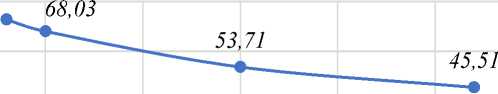
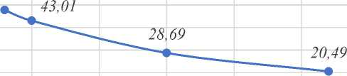
Figure 7 shows the change of cavitation pressure value over time when total G=0.42 m³/h, power =10 kW, and D=100 mm. The highest peak value is about 1730 KPa, the lowest value is about 562 KPa, and the range of pressure is about 1168 KPa.

Figure 8 shows the change of cavitation pressure value over time in scenario 2 when total G=0.42 m³/h, power =10 kW, and D=150 mm. The highest peak value is about 582 KPa, the lowest value is about 351.9 KPa, and the pressure range is about 230.1 KPa.

Figure 9 shows the change of cavitation pressure value over time in scenario 3 when total G=0.56 m³/h, power =10 kW, and D=100 mm. The highest peak value is about 2844 KPa, the lowest value is about 767 KPa, and the pressure range is about 2077 KPa.

Based on the above figure and the obtained data, using Scheme 1 as a reference, it can be found that:

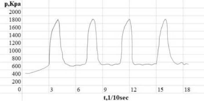
Figure 7. Instantaneous variation of pressure value after cavitation with time When total G=0.42 m3/h, Power=10 kW, D=100 mm

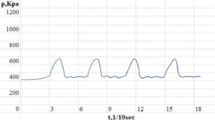
Figure 8. Instantaneous variation of pressure value after cavitation with time When total G=0.42 m3/h, Power=10 kW, D=150 mm

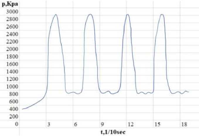
Figure 9. Instantaneous variation of pressure value after cavitation with time When total G=0.56 m3/h, Power=10 kW, D=100 mm

When the pipe diameter of Scheme 2 is approximately 1.5D 1 . During the closing period of the shock assembly, P 2 ≈ 0.34P 1 . Through calculation, it was found that a pipe diameter of 1.5 times can reduce the pressure to 0.34 times the original one. During the opening period of the shock assembly, P 2 ≈ 0.63P 1 , due to the presence of the shock assembly, the pressure change when it is opened is not as significant as when it is closed. it can be concluded that when the flow rate and output thermal power remain constant, the larger the pipe diameter, the lower the pressure, which is inversely proportional.

When the traffic of Scheme 3 is approximately 1.33G 1 . During the closing period of the shock assembly, P 3 ≈ 1.64P 1 . Through calculation, it was found that a pipe diameter of 1.33 times can increase the pressure to 1.64 times the original. During the opening period of the shock assembly, P 3 ≈ 1.36P 1 , due to the presence of the shock assembly, the change when it is opened is not as significant as when it is closed. It can be concluded that when the pipe diameter and output thermal power remain constant, the greater the flow rate, the greater the pressure, and the relationship is proportional.

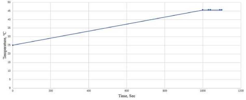
Figure 10. Diagram of temperature changes at the inlet and outlet when using a 10 kW cavitator, total G=0.42 m³/h, D=100 mm

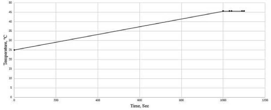
Figure 11. Temperature variation diagram of inlet and outlet when using two parallel 5 kW cavitators, total G=0.42 m³/ h. D=100 mm

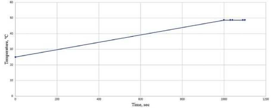
Figure 12. Temperature variation diagram of inlet and outlet when using three parallel 3.25 kW cavitators, total G=0.42 m ³/ h. D=100 mm

The above three figures show the temperature changes at the inlet and outlet of one 10 kW cavitation system, two parallel 5 kW cavitation systems, and three 3.25 kW cavitation systems when the total flow rate is 0.42 m3/h and the pipe diameter is 100 mm. As can be seen from the graph, these three graphs have one thing in common: the temperature gradually rises to a relatively stable state after 1000 seconds.

Table 6 shows the performance comparison of the three cavitation schemes, and discusses the comparison of pressure drop, temperature, heat transfer, efficiency and other parameters when the total output power is basically the same and different numbers of cavitation are paralleled. It can be seen from the data in the table that the pressure drops when the shock assembly is closed is larger than when it is opened. When the shock assembly is opened, the system with two 5kW schemes in parallel gets more heat energy than when it is closed, and the other two groups are basically unchanged. The three 3.25 kW cavitation units in parallel have a lower pressure drop, obtain the most heat energy and have a higher efficiency of converting electrical energy into heat energy.

Table 6

PERFORMANCE COMPARISON OF THREE CAVITATION SCHEMES
Cavitation scheme	Pressure, Kpa	Power, KW	Initial temperature, °C	System outlet temperature, °C	Q, J	η, %
Simulated data table when the shock assembly is closed
10 kW	1730	10	25	45.55	36.2502	0.363
Parallel connection of two 5 kW	1015.56	2×5	25	45.54	36.23256	0.362
Parallel connection of three     458 3.25 kW		3×3.25	25	48.62	41.66568	0.427
Simulated data table when the shock assembly is open
10 kW	562	10	25	45.55	36.2502	0.363
Parallel connection of two 5 kW	431	2×5	25	45.55	36.2502	0.363
Parallel connection of three    329.12 3.25 kW		3×3.25	25	48.62	41.66568	0.427

Figures 13 and 14 are derived from the data in Table 6. Because when the shock assembly is on, the system with the two 5 kW cavitation parallel scheme has an outlet temperature 0.01°C higher than when it is off, more heat energy is obtained. In the other two groups, the outlet temperature remained stable.

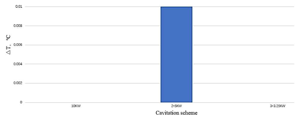
Figure 13. Shock assembly switch state Temperature difference at system outlet

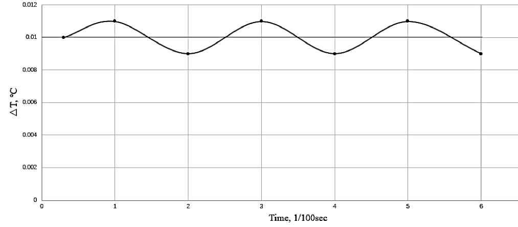
Figure 14. Temperature difference between the shock assembly switch states when using two parallel 5kW cavitators, total G=0.42m ³/ h. D=100mm

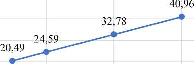
Figure 15 shows the change of temperature after cavitation and the change of temperature difference before and after cavitation with thermal power when pipe diameter is 100 mm and flow rate is 0.09m3/h. As can be seen from the figure above, when the thermal power increases from 5 kW to 10 kW, the temperature rises from 45.5°C to 65.98°C, and the temperature difference increases from 20.49°C to 40.49°C. Therefore, when the pipe diameter and flow rate remain unchanged, the greater the output thermal power, the greater the temperature and temperature change, and this relationship is proportional.

Бюллетень науки и практики / Bulletin of Science and Practice Т. 9. №9. 2023

Figure 15. The variation of temperature after cavitation and temperature difference before and after cavitation with power

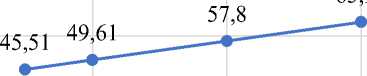
Figure 16 shows the temperature change after cavitation and the temperature difference before and after cavitation with the flow rate when the pipe diameter is 100 mm, and the thermal power is 10 kW. As can be seen from the figure above, when the flow rate increases from 0.18 m3/h to 0.42 m3/h, the temperature drops from 72.8°C to 45.5°C, and the temperature difference decreases from 47.78°C to 20.49°C. Therefore, in the case of constant pipe diameter and output thermal power, the greater the flow rate, the smaller the temperature and temperature change, and this relationship is inversely proportional.

In this paper, a three-dimensional model of the design circuit of the Water heating cavitation device is established and simulated in Hysys software. The relationship between temperature, pressure, and flow rate of the cavitation generator in a pulse cooling water circulation device was studied. The Control variates is used to simulate the transient changes of the pressure behind the cavitation generator and the temperature difference before and after the cavitation generator with time under different flow rates, pipe diameters and power conditions. Discussed the comparison of parameters such as pressure drop, temperature, heat transfer, and efficiency under the condition of basically the same total output power and different number of cavitation in parallel. The control variates is used to study the relationship between the temperature after the cavitation generator, the temperature difference before and after the cavitation generator, the flow rate and the output heat power. The following are the main conclusions.

When the flow rate and output thermal power remain constant, the larger the pipe diameter, the lower the pressure, which is inversely proportional. The pressure changes the least with time when total G=0.42 m³/h, power=10 kW, D=150 mm.

When the pipe diameter and output thermal power remain constant, the greater the flow rate, the greater the pressure, and the relationship is proportional. The pressure changes the most with time when total G=0.56 m³/h, power=10 kW, D=100 mm.

Бюллетень науки и практики / Bulletin of Science and Practice Т. 9. №9. 2023

u

72,8

0,05       0,1

0,15      0,2      0,25      0,3      0,35      0,4      0,45

4             6             8            10            12

Power, KW

4             6             8            10           12

Power, KW

G, m³/h

0,05      0,1

47,78

0,15      0,2      0,25      0,3      0,35      0,4      0,45

G, m³/h

Figure 16. The variation of temperature after cavitation and temperature difference before and after cavitation with volume flow rate

Conclusions

When the total output power is 10kW, the outlet temperature of the system gradually rises to a relatively stable state after 1000 seconds for different power cavitator schemes. The system with two 5 kW cavitation parallel schemes has a change in outlet temperature during the shock assembly switch state, while in the other two groups, the outlet temperature remains stable.

When the pipe diameter and output heat power are constant, the larger the flow rate, the smaller the temperature after the cavitator and the temperature difference between the front and back become smaller. When the pipe diameter and flow rate are constant, the smaller the output thermal power, the smaller the temperature after the cavitator and the temperature difference between the front and back become smaller.