Designing of a liquid cooler with a phase transition with a power of 5 kW

Бюллетень науки и практики / Bulletin of Science and Practice

UDC 624.139                                        

As the power density of electronic devices increases, efficient cooling systems become increasingly important to ensure their safe and reliable operation. Liquid cooling, especially using phase-change liquid coolers, has been shown to be an effective cooling method for high-power electronic devices [1–3].

This paper introduces a phase change liquid cooler designed to handle 5 kW power. To achieve this, we studied the dependence of flow rate, heat dissipation rate and pipe diameter on temperature differences between refrigerant and environment. First, we studied the relationship between flow rate and temperature difference and determined the optimal temperature difference for maximum cooling capacity. Secondly, we investigated the relationship between heat dissipation rate and temperature difference and determined the optimal temperature difference for maximum power processing capacity. Finally, we investigated the relationship between pipe diameter and temperature difference and determined the optimal pipe diameter for maximum cooling capacity and power handling capacity.

Our results show that the phase-change liquid cooler designed in this paper can effectively handle a power of 5 kW. Our study of the dependence of flow rate, heat dissipation rate and pipe diameter on temperature difference between refrigerant and environment provides important design parameters for achieving optimal cooling performance.

Installation diagram of simulation device

The research device is composed of evaporator, condenser and enhanced cooling circuit. A heating element is arranged on the evaporator, and a copper net is arranged in the lower part of the evaporator. Porous elements are arranged in the form of felt in several layers of copper net to resist steam. In the cooling loop, we have a shock assembly. The dual-channel heat pipe (DCHP) increases the distance of heat from gravity to more than 0.5 meters, corresponds to the high heat flow on the evaporating surface, and is a closed evaporative condensation system with separate channels for steam and liquid. The DCHP works as follows: Heat entering the area between the evaporator wall and the capillary hole through the evaporator wall causes steam to pass through the pipe into the condenser, as the heat source passes through the capacitor, the steam condenses into a layer of closed liquid, and under pressure, the steam is pumped through the capacitor into the compensation chamber. The circuit is closed by inserting a small hole in the evaporator. In the second circuit, the cooling carrier can be provided in both steady and pulse modes.

It calculates the heat transfer coefficient of the device. The heat exchange of the heat exchanger is calculated first. In the calculation, the heat transfer surface required for cooling the heat source is also determined to reach a certain temperature. The surface of the heat exchanger is in place. Heat exchange Heat exchange coefficient has been determined. Then the area of the evaporator and the heat transfer coefficient of the evaporator are calculated.

Both hydraulic and thermal characteristics were also studied in order to better understand the nature of the generating force and to determine the required parameters more precisely.

The circuit consists of three components and the main interest is an energy converter, which converts pressure into force and flow into velocity.

The TPM500 temperature regulator is used in heat-shrink equipment, thermal presses (used in thermal transfer), in homogenizers, dryers, in equipment necessary for the production of building materials, extruders and other equipment requiring temperature control.

A standard pressure gauge is used to measure excess, vacuum pressure of liquid and gaseous non-aggressive to copper alloys, non-viscous and non-crystallizing media with temperatures up to

150 T. The pressure gauge case as standard is made of steel, the mechanism is made of brass alloy. The principle of operation of pressure gauges is based on the dependence of the deformation of the sensitive element on the measured pressure. As a sensitive element, a Bourdon tube is used. Under the influence of the measured pressure, the free end of the tube moves and rotates the pressure gauge needle using a special mechanism.

The wing water meter SVK-15G is designed to measure the volume of water in water supply systems in accordance with GOST R 50601-93.

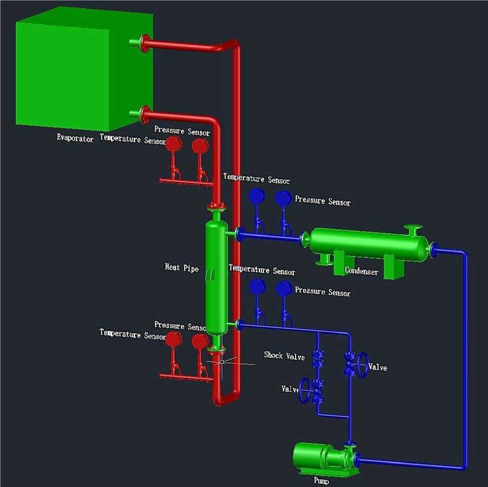
Figure 1. Simulation of steam heating and water condensation cycles in research facilities

Counters SVK-15G are universal and can be used to measure the volume of both hot and cold water.

The meter is used to record, including commercial, water consumption in the industrial and municipal sectors, as well as control technological processes.

Evaporator is a heat exchanger, in which the process of phase transition of the liquid coolant to the vaporous and gaseous state is carried out due to the supply from a hotter coolant. Such hot fluid is usually water, air, brine or gaseous, liquid or solid process products. When the phase transition process occurs on the surface of a liquid, this is called evaporation.

Simulation methods and programs

Hysys has an integrated engineering environment and is event-driven, so calculations can be done automatically, accurate results can be obtained, and all results can be scaled bidirectional to the entire process. Because of these characteristics of Hysys, this paper chooses Hysys as simulation software [4–6].

When planning the simulation, the following sequence of actions must be followed:

• -    Determine the number of experiments to remove transient function (t), amplitude-frequency A(Ω), phase-frequency φ(Ω) and static load characteristics;

• -    Determine when the transient or frequency response is first eliminated, as well as the total simulation time;

• –    Evaluate the influence of main factors on dynamic speed characteristics.

• –    Evaluate the influence of main factors on dynamic speed characteristics.

It is found that the sampling rate and bit depth of data acquisition have important effects on the measurement accuracy during the simulation evaluation of the calculation method of the characteristics of digital measurement tools. Therefore, the data file is recorded at several frequencies and the resulting bias is assessed [7–9].

In order to clearly determine the interrelationship between the temperature, pressure and flow of the heater and the condenser. We simulate the instantaneous change of pressure and temperature difference between heater and condenser with time under different flow rate, pipe diameter and power. Under a certain power, the temperature and temperature difference between heater and condenser are studied with the flow rate. Under a certain flow rate, we studied the temperature change after the heater and condenser cycle work and the temperature difference before and after the heater and condenser cycle work power.

Figure 2 is the Hysys simulation flow chart of 5 kW phase-junction liquid cooler.

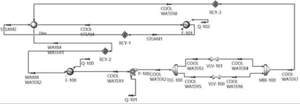
Figure 2. Hysys simulation flow chart of 5 KW phase-junction liquid cooler

Analog data processing

The simulation results are shown in Tables 1–4. The name label corresponds to the name in the simulation diagram.

Table 1

STATIC SIMULATION RESULTS WHEN TOTAL G=0.42 m3/h, power =10 kW, D=100 mm

Simulated data table when the shock walve is closed

Name	1	2	3	4	5
Temperature (°)	90	30	18.41	108.2	108.2
Pressure (kPa)	200	200	150	150	150
Molar Flow (kgmole/h)	16.65	16.65	11.10	11.10	0
Mass Flow (kg/h)	300	300	200	200	0
Liquid Volume Flow (m3/h)	0.3006	0.3006	0.2004	0.2004	0
Name	6	7	8	9	10
Temperature (°)	90.97	50.29	50.46	50.39	90.46
Pressure (kPa)	200	150	150	200	200
Molar Flow (kgmole/h)	16.65	16.65	11.10	0	11.10
Mass Flow (kg/h)	300	300	200	0	200
Liquid Volume Flow (m3/h)	0.3006	0.3006	0.2004	0	0.2004
Simulated data table when the shock walve is open
Name	1	2	3	4	5
Temperature (°)	90	30	18.41	108.2	108.2
Pressure (kPa)	200	200	150	150	150
Molar Flow (kgmole/h)	16.65	16.65	11.10	18.10	19.10
Mass Flow (kg/h)	300	300	200	180	240
Liquid Volume Flow (m3/h)	0.3006	0.3006	0.2004	0.1803	0.2404
Name	6	7	8	9	10
Temperature (°)	90	100	100	90	90
Pressure (kPa)	200	200	150	150	150
Molar Flow (kgmole/h)	33.12	33.12	33.12	13.32	23.31
Mass Flow (kg/h)	200	200	200	150	300
Liquid Volume Flow (m3/h)	0.3006	0.3006	0.3006	0.1002	0.2004

Simulation result diagram

According to the experimental data results in Tables 1–4, the curve of pressure changes with time before and after liquid cooling installation is drawn (Figure 3–5).

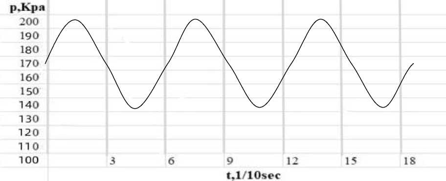
Figure 3. Instantaneous change of pressure value with time after liquid cooling Total G=0.42 m3/h, power =10 kW, D=100 mm

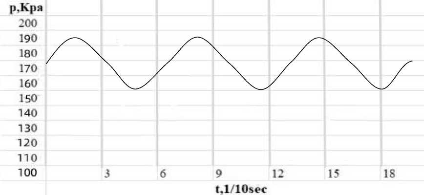
Figure 4. Instantaneous change of pressure value with time after liquid cooling Total G=0.42 m3/h, power =10 kW, D=150 mm

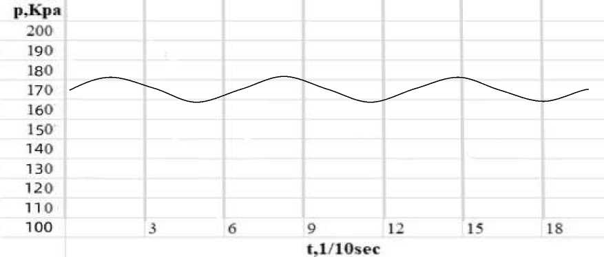
Figure 5. Instantaneous change of pressure value with time after liquid cooling Total G=0.56 m3/h, power =10 kW, D=100 mm

The above three P (t) plots use control variables. This is achieved by changing one of these variables, such as pipe diameter, flow rate, and power, while keeping the other two variables constant. As can be seen from the graph, these three graphs have one thing in common: they all belong to periodic wave curves. It can be seen that when the shock absorber assembly is closed, the pressure behind the liquid cooling reaches a peak state; when the shock absorber assembly is opened, the pressure after liquid cooling reaches a low state. It can be clearly seen that the pressure of option 3 changes the most overtime [10–12].

Figure 3 shows the change of liquefaction pressure value over time when total G=0.42 m3/h, power = 10 kW, and D=100 mm. The peak is about 200 KPa, the lowest is about 150 kPa, and the pressure range is about 50 kPa. Since the total G of scheme 4 is 0.42 m3/h, power =5 kW, D=100 mm, compared with scheme 1, only the heating power is different, and the influence of power on pressure is small and can be ignored. Therefore, the P(t) of scenario 4 is basically the same as that of Figure 4.

Figure 4 shows the variation of the spatiotemporal pressure value in scenario 2 with total G=0.42 m3/h, power =10 kW, and D=150 mm. The peak value is about 180 kPa, the minimum value is about 150 kPa, and the pressure range is about 30 kPa.

Figure 5 shows the change of cavitation pressure value with time in Scenario 3 when total G=0.56 m3/h, power =10 kW, and D=100 mm. The peak value is about 170 kPa, the minimum value is about 150 kPa, and the pressure range is about 20 kPa.

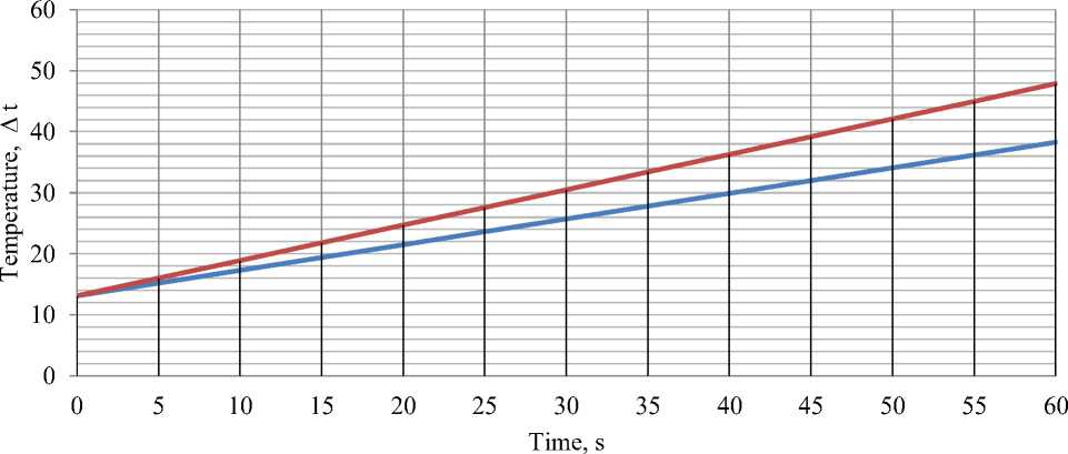
Figure 6. Graph of the difference in temperature of the coolant against time at a given flow rate of 0.42 m3/h with two different modes

Time, s

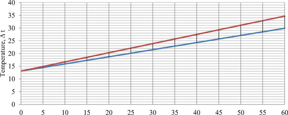
Figure 7. Graph of the difference in temperature of the coolant against time at a given flow rate of 0.56 m3/h with two different modes

Below are the graphs of the coolant to the heat pipe and at the output of the heat pipe (condensate) as a function of temperature versus time for 2 modes with different flow rates.

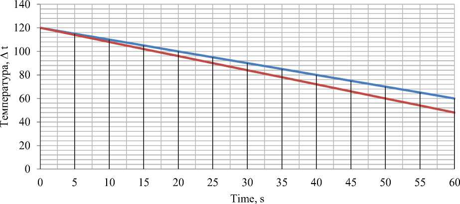
Figure 8. Graph of the difference in temperature of the hot coolant against time at a given flow rate of 0.42 m3/h with two different modes

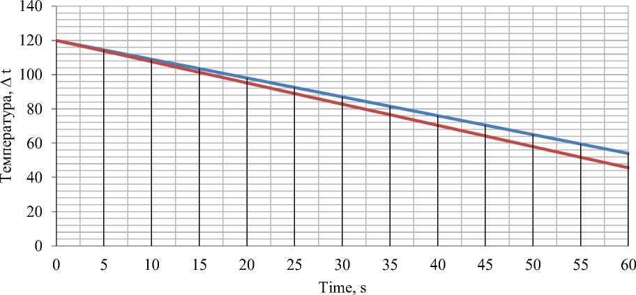
Figure 9. Graph of the difference in temperature of the hot coolant against time at a given flow rate of 0.56 m3/h with two different modes

Heat transfer coefficient calculation

We calculate the heat transfer coefficient in laminar and pulsed motion with different costs, thermal power, and the height of the nozzles.

The heat transfer coefficient is calculated by the following formula:

K экс =

dT λ× _dx

т _ пов

-

— охлж

Where: λ — thermal conductivity of the material; dT — temperature difference at the inlet and at the outlet of the coolant; dx — heat pipe length.

We carry out a series of experiments where the flow rate of the coolant, the height of the nozzles and the heating power change. Based on the data obtained during the first series of experiments, fill out (Table 2) in the Excel spreadsheet editor, construct a graph of the dependence of the heat transfer coefficient in 2 modes on the heater power and use the trend line function to determine the shape of the dependence

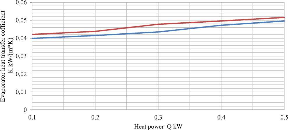
Figure 10. Graph of the heat transfer coefficient in two different modes on the heater power (flow rate of 0.42 m3/h).

Table 2

HEAT TRANSFER COEFFICIENT

	q 1	q 2	q 3	q 4	q 5
K stationary mode	0.03986	0.0415	0.0435	0.0472	0.0496
K pulse mode	0.0421	0.0438	0.0478	0.0496	0.0516

Figure 10 shows that the dependence of the heat transfer coefficient at two different modes on the heating power is a polynomial function of the following form:

y = -0.0001х3 + 0.0015х2 - 0.0021х + 0.0407

y = 0.0003x4 - 0.0036x3 + 0.0157х2 - 0.0244x+0.0541

Based on the data obtained during the second series of experiments, fill out (Table 3) in the Excel spreadsheet editor, construct a graph of the dependence of the heat transfer coefficient in 2 modes on the heater power and use the trend line function to determine the dependence.

Table 3

HEAT TRANSFER COEFFICIENT

	q 1	q 2	q 3	q 4	q 5
K stationary mode	0.0225	0.02456	0.0273	0.0321	0.0342
K pulse mode	0.0286	0.0312	0.0326	0.0361	0.0395

Бюллетень науки и практики / Bulletin of Science and Practice Т. 9. №10. 2023

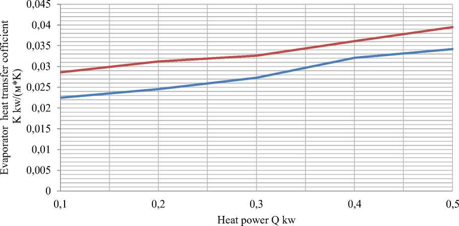
Figure 11. Graph of the heat transfer coefficient in two different modes on the heater power (flow rate of 0.56 m3/h)

Figure 11 shows that the dependence of the heat transfer coefficient at two different modes on the heating power is a polynomial function of the following form:

y = -0.0003х3 + 0.0027х2 - 0.0045х + 0.0247                           (4)

y = 0.00009x3 - 0.0006x2 + 0.0032х - 0.0259                           (5)

Conclusion

An information review on the research problem revealed that all heat pipes used in heat and water supply systems have limited use and have their advantages and disadvantages. The main advantages of a heat pipe include: lack of movable elements; silent in work; do not require additional energy sources for their work; have low thermal resistance; light weight per unit of transmitted power; a simple principle of action.

The calculation scheme for a prototype double-flow heat pipe with the ability to control the parameters of the working environment is developed.

The calculation setup allows you to implement the operation of the heat pipe in both normal and pulsed mode for subsequent comparison of efficiency when shooting experimental data.

We obtained data that allowed us to obtain the dependences of the heat transfer coefficient on the power of the heater, determined the heat transfer coefficient in the stationary and pulsed modes, obtained the dependence of the heat flux on the height of the lower part of the evaporator to the lower part of the heat exchange, on the maximum and minimum flow rate and heating power, as reducing flow rate, the outlet water temperature increases.

As a result of theoretical studies, it was found that the transmission coefficient of the heat pipe in the pulsed mode is 12% higher than in the stationary mode with the initial identical heat carrier parameters.

According to the results of the work, it is proposed to use the pulsed supply method as one of the ways to increase the heat transfer of a heat pipe.