Desirable Dog-Rabies Control Methods in an Urban setting in Africa -a Mathematical Model

Mathematical modeling has historically been of great importance in epidemiology and is a useful tool for providing a better insight into the dynamics of epidemic diseases such as rabies.

Rabies is a fatal, zoonotic, viral disease that causes an acute inflammation of the brain in humans and other mammals. It is transmitted by the saliva of infected animals via bites or scratches, with dogs being the primary source of transmission to humans [23].Rabies occurs in more than 150 countries and territories around the world and is most prevalent in developing countries in Africa and Asia [8].

Globally, it claims an estimated 60,000 human lives annually [15], the highest number of deaths caused by any zoonotic disease [11,16]. Dog transmitted rabies is estimated to cause 24,000 human deaths per year in Africa and [26] up to 60% of dog bite victims are children less than 15 years of age. Unfortunately, the majority of dog bites go unreported to parents and any resulting rabies cases are not reported to health authorities [2]. In Tanzania, it claims the lives of around 1500 people yearly [19].

The two main ways to control rabies transmission are mass-dog vaccination and culling, whereby the culling method is perceived to be easier and cheaper than vaccination, especially in the presence of free-roaming and poorly socialized animals in areas where veterinary personnel has relatively little experience or confidence in handling dogs [18].

Despite these control efforts, rabies remains a problem with 99% of all human deaths from rabies occurring in the developing world [14].

However, according to Mbwa wa Africa, an animal welfare organization in Arusha conducting research, every killed dog is replaced within 6 months by a new, young dog [22]. As dogs are territorial and defend their resting and feeding grounds in packs, killed members of a pack affect its ability to hold a territory, leading to more fighting and mixing of the overall dog population. Killing a neutered, vaccinated dog, therefore often leads to its replacement by an unvaccinated, unneutered dog, potentially increasing the risk for rabies outbreaks [22].

In order to reduce the risk of transmission and keep rabies control costs as low as possible, information on the efficacy of culling and mass dog vaccination programs is required. We used a mathematical model to establish the impact of culling and vaccination in Arusha respectively.

A similar model, but in a very different environment, was formulated to describe the dynamics of rabies transmission among dogs, livestock and humans within and around Addis Ababa, Ethiopia [8]. The model predicted an increase in rabies transmission with a maximum prevalence in 2024 and 2026 for both humans and livestock respectively and a combination of interventions was suggested. In another study, [12] a susceptible-exposed-infectious-vaccinated (SEIV) model for dog-human transmission of rabies considering domestic and stray dogs was proposed and showed that rabies in Guangdong province in China would decrease gradually before increasing again, indicating that in this case culling for disease control is futile. Differences in the dog populations, especially with regards to roaming patterns and contacts with wildlife areas require different modelling approaches to fit the conditions.

The specificity of our research considers three subgroups of dogs; domestic dogs with clear owners, stray dogs roaming the streets and Maasai dogs travelling alongside livestock and herdsmen. In this study, dog mass vaccination has been compared to stray dog culling in terms of its effects on rabies transmission risk.

• 2.    Materials and Methods

  • 2.1    Model Formulation

We developed a basic transmission risk model tailored to areas with similar settings as Arusha, to measure the effect of culling and vaccination. The formulated model has three dog subgroups, which are domestic dogs, stray dogs and Maasai dogs. Each population is categorized into Susceptible, Exposed, Infectious and Vaccinated individuals and a SEIV model was formulated.

The susceptible class consists of currently disease free individuals. The exposed class contains individuals who have been contracted the virus but do not show symptoms of the disease. The infectious class consists of individuals who were exposed to the disease, developed clinical symptoms of rabies and will die. Finally, the vaccinated class consists of individuals formally susceptible or exposed to the disease but now vaccinated. The formulated model is a system of differential equations, which has been derived from the compartmental diagram in Figure 1.

The model is developed based on the following assumptions; the susceptible populations are recruited via birth rate a. Any kind of dog which is exposed to bodily fluid from another dog is exposed. Dogs in each group have equal probability of dying a natural death. Populations are considered homogeneous with regard to each dog’s probability of being infected. Once a dog reaches the infectious stage, death is 100% certain. All parameters of the model are positive and they are introduced in table 1.

T able 1. P arameter D escription

Parameter	Description
« d . « s , d m 8 d , 8 s , 8 m	Annual births of domestic dog, stray dog and Maasai dog populations respectively. Death rate due to rabies for domestic dog, stray dog and Maasai dog populations respectively.
dd , ds, mm	The loss rate of vaccination immunity for domestic dog, stray dog and Maasai dog populations respectively.
Md > Ms > H m P d , P s , P m	Natural death rate of domestic dog, stray dog and Maasai dog populations respectively. Rate at which infectious stray dogs infect susceptible domestic dog, stray dog and Maasai dog populations respectively.
P d , P s , P m	The incubation period in domestic dog, stray dog and Maasai dog populations respectively.
^ d , ^ s , ^ m ^ md , T sd , V ds , Tra	Vaccination rate of susceptible domestic dog, stray dog and Maasai dog populations respectively. Number of dogs migrated from Maasai to domestic, stray to domestic, domestic to stray and Maasai to stray dogs' populations respectively.
M e	Average culling rate of stray dogs.

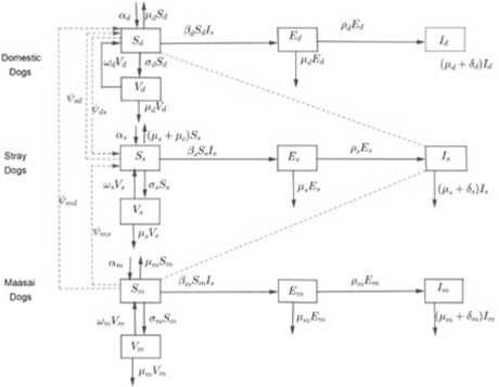
Fig.1. Flow diagram for rabies transmission among dog subgroups.

• 2.2    Model Compartment and Dynamics

2.3 Model Equations

From the above assumptions, definition of variables and parameters, the model flow diagram depicts the dynamics of rabies transmission among domestic dogs, stray dogs and Maasai dogs as shown in Figure 1.Parameters αi where, i = d, s, m represent annual births of domestic dog, stray dog and Maasai dog populations respectively. The parameters ρi where, i = d, s, m represent the latency rates of domestic dogs, stray dogs and Maasai dogs so that 1/ρi where, i = d, s, m are the corresponding incubation periods.

From the compartmental diagram we formulate a set of twelve differential equations as shown below:

<

d^=- = a, + mV, + V , + V , - V, - (u, + ст, + в I) Sd d d d sd md ds d d d s d dt dE- = PSA - (Ud + Pd)Ed dt dId" = PdEd - (Ud + 5,)Id dt dV

• - =- = ^ct-^s- ^- ( m ⁺ U ^)V d

dt s-—- = a + mV + V, +V -V,-(ст + и + и + BI )S s s s ds ms sd V s Us Uc г s s' s dt

• =    B s S s l s - ( U s + P s ) E s

dt di

• =    P s E s - ( U s + 5 s ) I s

dt dV

• V = CT s S s - ( ® s + U s V

dt

Г = d m + ® m^Vm ^{- V} ms ^{- V} md ^{- ( U} m + ^CT m + P m^-s ) ^Sm dt

• --=- = P m^Sm^-s - ^{( U} m ^{+ P} m ) ^Em

dt

• —= = ^P m^Em - ^{( U} m ^{+ 5} m ) ^-m dt

dVm

• = ^CT m^Sm - ⁽ ® m ^{+ U} m ^)Vm dt

with,

N d ( t ) = S d ( t ) + E d ( t ) + I d ( t ) + V d ( t ) N s ( t ) = S s ( t ) + E s ( t ) + I s ( t ) + V s ( t ) N m ( t ) = S m ( t ) + E m ( t ) + I m ( t ) + V m ( t )

Where N_t, i = d, s, m is the total of domestic dogs, stray dogs and Maasai dogs’ population at time t .

2.4 Invariant Region

The model represented by the system 1 of differential equations which deals with domestic dogs, stray dogs

and Maasai dogs, will be analyzed in the feasible region Φ and all state variables and parameters are assumed to be positive for all t≥0. The invariant region will be obtained through Theorem 1.

• Theorem 1

All solutions of the system 1 are contained in the region Ф £ M¹² and Ф = Ф_d U Ф_s U Ф_т

Proof

The model of the system 1 was grouped into domestic dogs N d , stray dogs N s and Maasai dogs N_m, such that

I

Ф d =Я S d , E d , I d , V d ) e □ + :0< N d < - d -J

I

I ф s = « Ss, Es, Is, Vs )e □ + :0 < Ns < - J

I

I

Ф m = « S m , E m , I m , V ) e □ + :0 <  N m <  - m J

(

And Ф is the positive invariant region for system 1. Thus,

ф = ф d иф s иф m e □ 4+x □ 4+x □ +

From that, it is sufficient to consider model system 1 in the region Ф, and it can be shown to be positively invariant. The model can be considered as epidemiologically and mathematically well-posed.

• 3.    Model Analysis

  • 3.1    Disease Free Equilibrium Points (DFE)

To find the disease free equilibrium points we set the right hand side of equations of system 1 equal to zero. In the absence of attack or in the absence of rabies, E d = I d = V d = E s = I s = E_m = I_m = V_m = 0. Then the disease free equilibrium (DFE) £₀will be £₀ = (S ° 0,0,0, 5 ° 0,0, E ? , S ^ , 0,0,0)

where

SO = -a — Tds +Уmd +Уsd , S0 =(Ms + ®s )(Tds -Tsd + Tms + -s ) , d          Md + Od        ’ s    Mc (Ms + ®s ) + Ms (Ms + ^s + ®s ) ,

• V0 =   -s (Tds +У ms + -s -Уsd )  , S0 = -m —^md —^ms

s   Mc (Ms + ®s ) + Ms (Ms + Os + ®s ) , m Mm + Om

The disease free equilibrium points for stray dogs populations that is Vs cannot be zero because once susceptible stray dog is vaccinated, it transfer to the vaccinated class. Hence the disease free equilibrium point of the system 1 exists and it is given by

£o =

«L

^- ds ^+- md ^+- sd ,0,0,0,

(Ms + ®s )(-ds --sd +-ms + «s )

V

Md + ^d

Mc (Ms + ®s ) + Ms (Ms + a. + ®s )

,0,0,

as (-ds + - ms + «s

- sd )   «m -- md

Mc (Ms + ®s ) + Ms (Ms + as + ®s ) ’    Mm + ^m

4х )

-ms - ,0,0,0

/

• 3.2    The Basic Reproduction Number R₀

The basic reproduction number R0 can be defined as the expected number of secondary infections produced by an index case in a completely susceptible population [24]. The basic reproduction number can be used to assess whether a newly infectious disease can invade a population [3]. R0 < 1 implies that, on average, an infected individual results in less than one newly infected individual during its infectious period, and the infection cannot grow. Conversely, if R0 > 1, on average, each infected individual creates more than one new infection, and the disease can raid the population. We used a next generation operator method proposed by Van den Driessche and Watmough (2000) [27].

We considered system 1 without vaccination i.e. to = a = 0. In this case we also do not have culling, which means цс = 0.

Let f i (x) be the rate of appearance of new infection in compartment i,v - (x) be the rate of transfer of individuals out of compartment i and v + (x) be the rate of transfer of individuals into compartment i by all other means, and it is assumed that each function is continuously differentiable at least twice in each variable. The disease transmission model of system 1 consists of non-negative initial conditions together with the following system of equations: X = F i (x) = f i (x) — V i (x)whereV i = v - — v + .We now consider expressions in which the infection is in progress. That is E d , I d , E_s, I_s, E_m, I_m

“T d" = P d S d I s ^- (M d ^{+ p} d ) E d dt

^7" = PdEd - (Md + §d)Id dt

= P.S.I, - (Ms + Ps)Es dt

dT = PsEs - (Ms + 5 )Is dt

• —=~ = P m S m I s ^{- ( M} m ^{+ P} m ) ^Em dt

• —=■ = PmEm - (Mm + 5m )Im

dt

By rearranging equations of system 1 without vaccination from exposed to infectious classes of dogs’ subgroups with a system of equations given by 7. Let F be a non-negative n X n matrix and V be a non-singular N-matrix such that dfi ( £0 ) xj

and V =

^^ ( £ о)

x j

with 1 < i, j < n.The point e ₀ is the disease free equilibrium point in 6 without vaccination where

■ P d S d I s " 0 f _ P s S s l s 0 P m SJ s _ 0 _

( P d + P d ) E d ( p d + 5 d ) I d - P d E d and v,=    . ( P s + P s ) E s                                                                 (9) ( P s + 5 s ) I s - P s E s ( P m + P m ) E m _ ( P m + 5 m ) I m - P m E m _

We consider classes in which the disease is in progress. Using the linearization technique, we get the Jacobian matrices of / and v at the disease free equilibrium point Eoas shown below:

0 0 0 F = 0 0 L o V - 1 =

0 0 P d a -^ ds +^ md +^ sd ) 0 0 " P                г 0 0             0             0 0        P d + P d      0       0       0       0        0 в (a +^+^—^)          — P d   P d + 5    0    0     0     0 0 0 '-------------- sd ) 0 0          0       0     P s + P s     0       0        0 P s                 ’ V = о        o     - P   P + 5    о        o 0 0             0             0 0          A       A       A       A                 A ,               .                     0        0        0       0      P m + P m     0 0 0     A m l ^ m zZ mi ZJ m l   0 0      L 0      0      0      0      - P s    P m + 5 m P m 0  0              0              0  0 _ ---1--- 0             0             0              0              0 P d + P d , - P'P*; p - p- , -1-        0          0           0           0 ( P d + 5 d )( P d + P d )   P d + 5 d 0         0      —1—      0         0         0 P s + P s 0            0    7---- -^s ------г                  0             0 ( P s + 5 s )( P s + P s )   P s + 5 s 0              0             0             0          ---1--- 0 P m + P m 0000 , _ Pm . . L                                                           ( P m + 5 m )( P m + P m )   P m + 5 m J

(10) (11)

We now multiply F and V ¹ and then compute the Eigen values of the resulting matrix FV ¹ and choose the maximum Eigen value as the basic reproduction number R_o which is given by

PsPs (Уds +У ms + as -Уsd ) Ps (Ps + 5s )(Ms + Ps )

• 3.3    Effective Reproduction Number R_e

The effective reproduction number Recan be defined as the average number of secondary cases that one index case generates over the course of its infectious period [7]. The prevalence of infection increases or decreases according to whether Reis greater than or less than one, respectively [6]. Here we consider the presence of control methods. In our case we have vaccination and culling. In this case to, цс and a will not take on zero values. So we include them and follow the same procedures usedin computing R0 and this will result in the spectral radius (dominant Eigen value) Re = pFV-1of FV-1given by

R e =

PsPs (Ms + ®s )(Y ds + У ms + as -Y sd )

(Ms + 8s ) (Ms + Ps ) (MA + MsMc + Ms^s + Ms®s + Ms )

Numerical computations of R0 and Re were done using the data collected from Mbwa wa Africa and the Ministry of Agriculture, Livestock Development and Fisheries of The United Republic of Tanzania.

T able 2. V alues of parameters used at DFE

Parameter		Value (year-1)	Source
« s	The annual births of stray dogs	2.5 x 10 2	[22]
8 s	Death rate due rabies for stray dogs	0.22	[4]
^ S	Loss rate of vaccination immunity for stray dogs	0.1	Assumption
P s	Natural death rate of stray dogs	0.32	[20]
U s	Rate of infection of stray dogs	1.7864 x 10-4	Data
P s	The incubation period of stray dog	0.83778234	[17]
" s	Vaccination rate of the susceptible stray dogs	0.25174	Data
^’ms	Average number of Maasai dogs that migrate to stray dogs population	35	Fitting
^ sd	Average number of stray dogs that migrate to domestic dogs	17	Fitting
	population
^s	Average number of domestic dogs that migrate to stray dogs	56	Fitting
	population
P c	Average culling rate of stray dogs	0.01792	Data

We now substitute the parameter values to the expression found in 12 and 13 to have

1.7864x10 — 4 x0.83778234x ( 56 + 35 + 2.5x10 ² -17 ) ---------------;-------------      --------------------;------- » 1.9

0.32 x ( 0.22 + 0.32 ) x ( 0.32 + 0.83778234 )

Without any control measure the result of R0 is greater than one which shows that the disease will invade the population.

Re =

1.7864 X10 ^{- 4} x 0.83778234 x0.42 ( 56 + 35 + 2.5 x10 ² -17 ) 0.54 x 1.15778234 ( 0.001792 + 0.0057344 + 0.0805568 + 0.032 + 0.32 2 )

«1.2

With the current vaccination coverage, Re is more than one and this shows that the disease still perseveres. This implies that more efforts should be taken to fight against rabies transmission. We have simulated the effective reproduction number with some variations in vaccination coverage and a combination of vaccination and culling methods. It shows that, by increasing the vaccination of stray dogs, there is a possibility of rabies to die out. The combination of vaccination and culling was found to be the best way to fight against rabies disease transmission in Arusha town. In the simulation, R0 is without any control, Re1 is the current 25% vaccination coverage, Re2 is the 40% vaccination coverage and Re3 is the combination of 60% vaccination coverage and 40% culling.

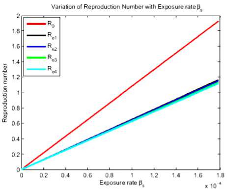
Fig.3. Reproduction number for different culling coverages

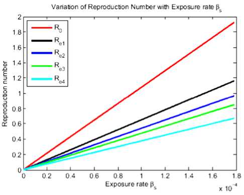
Fig.2. Reproduction number for different vaccination coverages and combination of vaccination and culling.

From Figure 2 we can see that Re3 < Re2 < Re1 < R0. This indicates that if we increase vaccination in the stray dog population, the effective reproduction number decreases and become less than one. Due to the high transmission rate of rabies from stray dogs to domestic dogs and Maasai dogs, combination of measures is eagerly recommended as it makes the effective reproduction number less than one. In this case R0 is the current 40% culling of stray dogs, Re1 is the 50% culling, Re2 is the 60% culling and Re3 is the 70% culling whereby the 25% current vaccination rate is kept constant.

From Figure 3 we see that culling alone has got a very minute impact in combating rabies transmission risk. The effect observed is for 25% vaccination coverage only. Therefore, if other practicalities such as costs are disregarded, using a combination of vaccination and culling to control rabies transmission has the highest impact, with increased vaccination coverage.

• 4.    Stability Analysis

  • 4.1    Local Stability of the Disease Free Equilibrium Points

Theorem 2

If R_e< 1 , then

• •    The disease-free equilibrium e₀ of system 1 is locally asymptotically stable;

• •    The disease-free equilibrium e₀ of system 1is globally asymptotically stable in the region Ф

Next we derive the Jacobian matrix of system 1 by differentiating each of the equation of system 1 in terms of state variables S_d, E_d, I_d, V_d, S_s, E_s, I_s, V_s, S_m, E_m, I_m, V_m at the disease free equilibrium point from 6 to have

-(Md + ®d) 0 0 % 0 0 A 0 0 0 0 0 " 0 H 0 0 0 0 B 0 0 0 0 0 0 Pd -(Md + 5d) 0 0 0 0 0 0 0 0 0 ^d o 0 -(Md + md) 0 0 0 0 0 0 0 0 0 0 0 0 G 0 C ®s 0 0 0 0 J = 0 0 0 0 0 — (Ms + Ps ) D 0 0 0 0 0 ^0 0 0 0 0 0 Ps —(Ms + 5s) 0 0 0 0 0 0 0 0 0 ^s 0 0 I 0 0 0 0 0 0 0 0 0 0 E 0 -(Mm + CTm ) 0 0 % 0 0 0 0 0 0 F 0 0 J 0 0 0 0 0 0 0 0 0 0 0 Pm -(Mm + 5m ) 0 .      0 0 0 0 0 0 0 0 ^m 0 0 K _ (16) where

,  -в («d -Vds + Vmd + Vsd ) R  Pd (»d -^ds + Vmd + Vsd )

A =, B =, Md + ^d                      Md + ^d

C _"P, (Ms + to )(V ds -V sd +V ms + «s ) D = Ps (Ms + to )(V ds -V sd + V ms + a )

Mc (Ms + ®s ) + Ms (Ms + ^s + ®s )   ’ Mc (Ms + ®s ) + Ms (Ms + ^s + ®s )

p -Ps (am -V md +V ms )     Ps (am -V md + V ms )

E = -----------,----------- , F = ----------,----------- , G = -( M s ⁺ P s ) ,

Mm + ^m                Mm + ^m

H= -(Md + Pd ) , I = -(Ms + ®s ), J = -(Mm + Pm ) , K= -(Mm + ®m )

The Eigen values of the Jacobian Matrix are:

^- ^ d - ^M d

-Md

-8

-

M

- M _m

-

■ M d

-

P d

^- M

-

P m

—

P s ) ^{2 - 8} s ^{- 2} M s ^- P s

—

^p s ) ^- 8 s ^- 2 ^M s ^{- p} s

^-M d ^{- CT} d

-

® d

^- M,

-

m

-

to

m

CT s ⁺ M c ) ⁺ ® s

-

² M s

-

s

-

CT s ⁺ M c ) ⁺ ® s

-

2 M s

-

s

-

From the above Eigen values we see that they are all negative but if

^4DPs +(5s - Ps )2 < 8s + 2Ms + Ps and

• 4.2    Global Stability of Disease Free Equilibrium Points

In this case we employ the method suggested by [19] to scrutinize the global stability of disease free equilibrium point of system 1.Our model represented in system 1 has the following structure.

dx j

-5 = A (x dy

। ft = A 2 y

<

- x_£

^E 0

) + A 1 У

■ S d "	■ E d 1
V d Ss	, У =	I d E s	and x
V s S m _ V m _		I s Vm [ I m j	‘

Where; x £ K + standsforsusceptible and vaccinated individuals. у £ K + stands for exposed and infectious individuals. x_Eo is a vector at DFE point £₀ of the vector length x. With reference to the system 1 we define

■      « d -Y ds + Y md + Y sd     1	^ x - xr = = 0	■    s    a d -Y ds +Y md +Y sd     1	(22)
^ d + ° ( M s + « s )( Y ds -Y sd + Y ms + a )		S d - M d + O d V d „  ( M s + « s )( Y ds -Y sd +Y+ a s )
M c ( M s + « ) + M s ( M s + O s + « ) a s ( Y ds -Y sd +Y ms + a s )		“ s    M c ( M s + « s ) + M s ( M s + O s + « s ) a YdS-Ysd-vYms-v a) V           s     ds      sd      ms     s
M c ( M s + « ) + M s ( M s + O s + « ) a m -Y md -Y ms		s   M c ( M s + « s ) + M s ( M s + O s + « s ) C      m     md     ms
Ц + CT Mm   m _                        0                        .		m      M m + O m .                      V m                     .

To test for global stability of the disease free equilibrium we need to prove the following;

• •    А should be a matrix with real negative Eigen values,

• •    А 2 should be a Metzler matrix.

Using system 1 together with the representation in 21 the two equations can be written as shown below.

ad + ®dVd + Ysd + Ymd - MdSd - ^dSd -Yds - PdSdIs ^dSd - ®dVd - MdVd a + ®V + Y, +Y - у S - (m + m )S -Y,-BSI s s s ds ms s s   Wss   Mc / s sd ss s s у S - ®sVs - UsVs am + ®mVm - MmSm -Yms -Ymd - УmSm - PmSm1 s CTmSm - ®mVm - MmVm

P d^Sd I s - ( M d ⁺ P d ) ^Ed P a^Ed - ( M d ⁺ P i ) I d P s S s l s - ( M s + P s ) E s P s^Es - ( M s ^{+ 5} s ) I s P m^Sm I s -^{( M} m ^{+ P} m ) ^Em ^P m^Em -^{( M} m ^{+ 5} m ) I m

= A 2

E d I d E s

s

V m

m

„ a, - Y, + Y , + Y , d ds md sd

^Sd                   i

M d ^{+ y} d

V d

S   ( M s + ® s )( Y ds -Y sd +Y ms + a s )

s   Mc (Ms + ®s ) + Ms (Ms + ^s + ®s )

V - a s ( Y ds -Y sd +Y ms + a s ) s M c ( M s ⁺ ® s ) ⁺ M s ( M s ⁺ ^ s ⁺ ® s )

⁺ A i

E d I d E s

s

V m

MatricesA, A 1 and A 2 are of order 6x6. Using elements of x of the Jacobian matrix of system 1 at £ 0 and representation in 21 we get

	-( M d + ° a )	® d	0	0	0	0      1		" 0	0	P d S d	0	0	0 "
	y d	- ( ® d + y d )	0	0	0	0		0	0	0	0	0	0
A =	0	0	-( M s + M c )	® s	0	0	, A i =	0	0	e s s s	0	0	0
	0	0	y s	-( ® s + M s )	0	0		0	0	0	0	0	0
	0	0	0	0	-( M m + y m )	® m		0	0	P m S m	0	0	0
	0	0	0	0	y m	-( ® m + M m ) _		. 0	0	0	0	0	0 _
	-( M d + P d )	0	0	P d S d	0	0      "
	P d	-( M d + y d )	0	0	0	0
Л =	0	0	-( M s + P s )	e s s s	0	0
2	0	0	P s	- ( M s + 5 s )	0	0						(24)
	0	0	0	P m S m	-( M m + P m )	0
	0	0	0	0	0	-( ® m + 5 m ) _

Now we have deduced that, matrix A is an upper triangular matrix with Eigen values being real and negative located in its main diagonal. The Eigen values are - (n d + p d ), - (n d + a d ), - (n s + p s ), - (n s + S s ), - (ц_т + p m ) and - (ц_т + S m ). The off diagonal elements of matrix A 2 are non-negative since all parameters are positive which proves that it is a Metzler matrix. This also shows that the disease free equilibrium points of system 1 is globally asymptotically stable in the region Φ. This brings us to the following crucial theorem.

Theorem 3

The disease free equilibrium point is globally asymptotically stable in the region Ф if R e < 1 and unstable in the region Ф if R e > 1 .

• 5.    Endemic Equilibrium Points

  • 5.1    Existence of Endemic Equilibrium Points

We equate the right hand side of system 1 to zero to be able to compute the equilibrium points of system 1. If the endemic equilibrium points of system 1 exist, they are given by

*    I с*       т*  гл*               гл*                 гл*\

^ =( Sd, Ed, Id, Vd , Ss, Es , Is , V , Sm, Em, Im, Vm)

where

T7-* IT,      IT,       IT,                 /1 T*CT*

• o* _ ad + todVd — ^ds +^ md +^ sd p * _ PdIsSd  T * _ PdEd     * _

S d =              nr*             , E d =         , I d = c , V d =

Vd + PdIs + a.              Vd + Pd      Sd + Vd       Vd as + tosV -^ sd +W ms +W ds ^  Psi’s SS

---------------ST-----------, Es =,

Vs + Vc + в sis + ^s           Vs + Ps am + tomVm -^ ms +^ md n* _ PmIsSmr*

■ --------------, „ .* ,--------------, Em = -------,,

V m ^{+ P} m I s ⁺ ^ m           V m ⁺ P m

_ .^EL, V _ ^S(27)

S _s + V _s         V _s + to _s

PmEm   V*   ^mSm(28)

• ^S m ⁺ V m ’ m    V m ^{+ to} m

Local Stability of the Endemic Equilibrium

We employed the following theorem as explained by Paul et al., (2016) [20] to describe and prove the local stability of the endemic equilibrium points of system 1.

Theorem 4 (Routh-Hurwitz Criterion )

Given a polynomial P(A) = Л ” + d 1 A^n- 1 + —+ d_n-1A + d_n

- ( V d + °"d + P d I s )        0             0 _       P d I s        - ( V d + P d )       0 J £ 0 =         0               P d      - ( V d + S d )

to d      " 0 0                                         (30)

-(Vd + tod)

Where the coefficients d j are real constants, i = 1,.., n define the n Hurwitz matrices using the coefficients d j of the characteristic polynomial:

a 1 r            a,   10          ал Г 1              a 1      1                  1                                      3 H 1 = [ a l ] , H 2 =          , H 3 = a 3 a 2   a l ,-, H n = a 5 a 3    a 2	10 0 - 0" a 2 a 1   1    —    0 a 4 a 3   a 2   —   0
a 5    a 4    a 3                   : 0	:       :       :      \      : 0   0   0 — a n J                  (29)

Note that, a i= ₀ifj > 0. All of the roots of the polynomial P(A) are negative or have negative real part if the determinants of all Hurwitz matrices are positive: det H j > 0; j = 0,1,2, .„, n. More details on Routh-Hurwitz criterion are given by Paul et al., (2016) and Sambo et al., (2013) [21,22]. Consider the first part of system 1. The Jacobian matrix of that part is given by

Through computations, we derive the following characteristic polynomial.

P (X) = X4 + AX? + BX1 + CX + D                                                         (31)

A = ³ d ⁺ 4 M d + ^p d + P d I s ⁺ C d + to d

^B = ^{3 3} d M d ^{+ 3} d ^p d ^{+ 3} d ° d ^{+ 3} d ^to d ^{+ 3 p} d M d ^{+ 3 M} „ c „ ⁺ 3 Md ^tod ^{+ 6} М 2 ^{+ p} d ° d ^{+ p} d ^to d ⁺ I s P d S d + ³ I s P d M d ⁺ I s P d ^p d

+ PPdtod + Odtod

^C = ^{2 3} d M d P d ^{+ 2 3} d M d ^ d ^{+ 2 3} d M d to d ^{+ 3 3}d M d ⁺ 3 d P ^{0 +} S d ^ d to i ⁺ 3 d P ^{to + 2} M d P ^{0 + 2} M d P d ^to d ⁺ VdPd ⁺

• ^{2    M} d ^O d ^to d ⁺ 3 ^Md^ad ⁺ 3 ^Md^tod ^{+ 4 M} d ⁺ P d ⁰ ! ® ! ^{+ 2} I s P d S d ^M d ⁺ I s P d ³ d ^p d ⁺ I s P d ³ d ^M d ^to d ^{+ 2} I s P d ^M d ^p d ⁺

• 2    I s P d M d to d + 3 I s P d M d + I s P d P d M d

D = 3d Md Pdcd + 3d Md Pdtod + 3d Md Pd + 3d Mdcdtod + 3d Mdcd + 3d Mdtod + 3d Md + 3d Pdcdtod + Md Pdcdtod + Md PdCTd +Md Pdtod + Md Pd + Mdodtod + Mdod + Mdtod + Md + IsPd3d Md Pd + IsPd3d Mdtod + IsPd3d Md + IsPd3d Pdtod + IsPdMd Pdtod + IsPd Mdtod + IsPd Md

From the characteristic polynomial represented in 31 we have the following Hurwitz matrix

A 100

CBA 1

0 DCB

000 D

The determinant of the Hurwitz matrix is D (ABC — C² — A² D).

From the Routh-Hurwitz criteria of Theorem 4, we see that the determinant of Hurwitz matrix will be positive if the following conditions hold true. A > 0, C > 0, D > 0 and ABC > C2 + A2D .Recall that all parameters of our model and all coefficients of the characteristic polynomial are positive as shown in equation 32. We combine all requirements and deduce that all roots of the polynomial represented in 31 are negative and hence we prove that the first part of system 1 is locally asymptotically stable. Moreover, we consider the second part of system 1. The Jacobian matrix is given by

	- ( ° s + M s + M c + P s I s )	0	P s S s	to s
J \ ^ 0 =	P s I s 0	- ( M s + P s ) P s	- P s S s - ( M s + 3 s )	0 0
	_            ° s	0	0	-( M s + to s )_	(34)

Consider the characteristic polynomial

P (X) = X + Aj23 + Bj22 + C1X + D1

A1 = Цс + PsIs + 3s + 4 Ms + ps + ^s + ®s

B1 = Mc3s + McPs + Ma + 3MCMS + PsIsSs + 3PPM + PsIsPs + 33SMS + 5sPs + 3 ® + 3a + 3MsPs

• +    3M^S + 3M a + 6M2 + P®. + Pa - PsPsSs

• C 1 = Mc3sPs + Mc3s®s + 2MC3SMS + McPs®s + 2MCMPS + 2 M.Ma. + 3MCM2 - McPsPsSs + 2 A Is 3sMs +

• +    PsIsSsPs + PsIs5s^s + 2p IsMsPs + 2PS IsMs^s + 3PS Is M2 + PsIsPs^s + 23sMsPs + 'pM® + 23sMsas + 33sM2 + 3pG. + 3spsas + 2msp^s + 2m P a + 3^2ps + 3м2- + 3Ms2as + 4^3 -      (36)

• 2    PsMsPsSs — PsPs^sSs — PsPsSs®s

D1 = Mc5sPs®s + Mc5sMsPs + Mp3.Ma. + Mc3sM2 + McMsPs^s + McM2 Ps + McM^s + McM2 — M,P.PS®.

• - McPsMsPsSs + PsIsSsMsPs + PsIs5sMs®s + PslsSsMs + PsIs5sPs®s + pi M p® + PsIsM2Ps + psIsMsas + psIsH + Spispn. + 3sMsPsas + 3sMs Ps + SsMs^s + SsMsas + SsMs + Ms Ps^s + Ms Ps®s

+ Ms3Ps + M>s + M2®s + Ms4 - PsMsPs^sSs — PsMsPsSs®s — PsM2PsSs

From the characteristic polynomial represented by 35 we have the Hurwitz matrix being given by

A1  1  00

C 1 B 1 A 1 1

0  D1C1B1

000D1

The determinant of the Hurwitz matrix is given by D₁(A 1 B₁C 1 — C 2 — A 2 D 1 ). With reference to Theorem 4 the determinant of Hurwitz matrix become positive iff A 1 > 0, C 1 > 0, D 1 > 0 and A 1 B 1 C 1 > C 2 + A ^ D 1 . Again, since A 1 > 0,

B 1 >  0 iff M c ⁵ s + M c P s ⁺ M c ® s ⁺ 3 M c M s ^{+ I}s P s 5 s + 3 I s P s M s + I s P s P s + I_S P _S ® _S + ^{3 5} s M s + S s P s + 3 _s ct _s +

⁵ s ® s ^{+ 3} M s P s ^{+ 3} M^_S ^{+ 3} МЖ ⁺ 6 M 2 ⁺ P _s ct _s + P s ® s > P s P s S s

C 1 >  ⁰ iff M c ⁵ s P s ⁺ M c ⁵ s ® s ^{+ 2}Me ⁵M_S ⁺ M c P s ® s ^{+ 2} MMP_S ^{+ 2} McM^_S ^{+ 3} Mc ^{p2 + 2} I s P s P s M s ⁺ I s PAP s

+ I ps a + 2 I s P s H s P s + 2 1 в Ц a + 3 I s P s M s + I в P® + 2 3_SM_SP_S + 2 3_SH^_S + 2 3^^,, +

^{3 5} s M s 2 ^{+ 3} s P _s CT _s + ³ s P s ® s + 2 U P® ^{+ 2} H_SP®_S ^{+ 3} M s 2 P s ^{+ 3} M s ^! CT s ^{+ 3} M s -®_s ^{+ 4} M s ³ >  ^{2 p} MP _sS_s ⁺        (38)

pP- S ^{+ p} s P s^Ss ^a s ⁺ H c ^p s P s^Ss

D 1 >  ⁰ iff H c ³ s P s ^a s ⁺ H c ³ s H s P s ⁺ H c ³ s H s ^a s ⁺ H c ³ s H^{2 +} H c H s P s ^a s ⁺ H c M 2 P s ⁺ H c H^2a s ⁺ H c M s ^{+ I}s ^p s ³ s H s P s

+ I s p s S s M s a s + I s p s S s M ² + I s p s P s P s a s + I s p s M s P s a s + I s p s M s P s + I s p s M ² ® s + I s p s M ³ + sup®

^{+ 3} s M s P s ^a s ^{+ 3} s M²® s ^{+ 3} s M^2a s ^{+ 3} s M s P s ^{+ 3} s M s ⁺ M s P- s ⁺ M s P s ^a s ⁺ Ms³ P s ⁺ M²® _s ⁺ M s ^a s ⁺ M s

• > pLm^p® ^{s + p} s M s P s S s ^a s ^{+ p} s M s P s S s ⁺ M c ^p s P s^Ss ^a s ⁺ M c ^p s M s P s^Ss

• 6.    Conclusion

When all conditions hold, similarly A 1 B 1 C 1 > C 2 + A ^ D 1 holds. Hence we can conclude that all roots of polynomial 35 are negative. This verifies that the second part of system 1 is locally asymptotically stable. Using the same procedure for the third part of system 1 will result in the same conclusion.

Therefore, we generally conclude that the endemic equilibrium point of system 1 is locally asymptotically stable.

In this paper we have formulated and analyzed a deterministic mathematical model for the dynamics of rabies transmission. The model consists of domestic dogs, stray dogs and Maasai dogs’ population. The model intended to show the contribution of vaccination, culling and their combination towards the control of rabies transmission.

The basic reproduction number and the effective reproduction number have been computed using next generation matrix operator. The results depend on the parameter values of stray dogs’ population. This is because, epidemiologically, stray dogs are the main source of dog-rabies transmission. This tells us that more effort on controlling dog-rabies transmission should be put into the stray dog population [12].

Using our set of parameter values, the basic reproduction number R0 and the effective reproduction number Re were computed and found to be 1.9 and 1.2 respectively. This indicates that the disease is endemic [8].

The numerical simulation for the reproduction number indicates that the combination of at least 60% vaccination and culling of up to 40% of the dog population would be the best measure to control dog-rabies transmission in Arusha region. However, this does not take into account feasibility and economic and sociocultural aspects.

We have computed the disease free and endemic equilibrium points. With the use of Routh Hurwitz criteria, the endemic equilibrium points are locally asymptotically stable if these conditions hold.

Acknowledgments

The authors thank MWECAU for the sponsorship of studies. Also authors appreciate the data provision support from the ministry of agriculture, livestock development and fisheries of the United Republic of Tanzania and Jens Fissenebert of Mbwa wa Africa.