Despeckling of Medical Ultrasound Images: A Technical Review

Автор: Nidhi Gupta, A.P Shukla, Suneeta Agarwal
Журнал: International Journal of Information Engineering and Electronic Business(IJIEEB) @ijieeb
Статья в выпуске: 3 vol.8, 2016 года.
Бесплатный доступ
Acquisition of digital image and preprocessing methods plays a vital role in clinical diagnosis. The ultrasound medical images are more popular than other imaging modalities, due to portable, adequate, harmless and cheaper nature of it. Because of intrinsic nature of speckle noise (signal based noise), ultrasound medical image leads to degradation of the resolution and contrast of the image. Reduction of this signal based noise is helpful for the purpose of visualization of the ultrasound images. The low quality of image is considered as a barrier for the better extraction of features, recognition, analysis and detection of edges. Because of which inappropriate diagnosis may be done by doctor. Thus, speckle noise reduction is essential and preprocessing step of ultrasound images. Analysts survey manifold reduction methods of speckle noise, yet there is no exact method that takes all the limitations into account. In this review paper, we compare filters that are Lee, Frost, Median, SRAD, PMAD, SRBF, Bilateral, Adaptive Bilateral and Multiresolution on medical ultrasound images. The results are compared with parameter PSNR along with the visual inspection. The conclusion is illustrated by filtered images and data tables.
Despeckling, speckle noise, filtering mechanisms, wavelet thresholding
Короткий адрес: https://sciup.org/15013417
IDR: 15013417
Текст научной статьи Despeckling of Medical Ultrasound Images: A Technical Review
Published Online May 2016 in MECS
In the field of medical science, as the human’s body visual representation process upgrading as well as increasing day by day, amid all of them, ultrasound images are supposed to the most portable, non-invasive, accurate and non-toxic to the human body. These characteristics of ultrasound images, make it famous amid all the hospitals and thus adequate diagnosis is done by the doctors. Despite of its usefulness, the image quality degrades due to many factors in which speckle noise is the one that we are considering as the responsible factor. The speckle noise destroys the image details such as quality, contrast, preserving edges etc. Thus, the presence of speckle noise lacks the observer to diagnose the problem, effectively. Thus, manifold efforts have been taken into account in order to reject the speckle noise, known as despeckling methods.
Speckle noise is an inherent property of ultrasound images and the images are designed by intrusion sounds of a wave that is transmitted and comes from different regions of an observed body part. All these sounds are superimposed with different amplitudes as well as phases, results in producing a complex intrusion pattern, known as speckle noise. This noise limits from minimum to maximum, totally based on its intrusion type (constructive or destructive). As we have to study about human tissues, speckle noise leads to degrade the beneficial details, thereby the problem will not be properly diagnosis. The analysis of statistical property of speckle noise that is given by Goodman [1], helps in rejecting of it and initially take laser speckle into consideration. In addition to this, Goodman also provides the way to suppress the speckle noise via filtering (linear) and results in improving the quality of the image. The statistical property of this type of noise helps in discriminating, among the kind of biological tissues [2] [3]. The outcomes of [1] were updated in [2]. As a conclusion, it was observed that in [1], the use of linear filter leads to, over smooth essential contents in the image. In order to overcome this drawback, an adaptive median filters [4] [5] which were also not appropriate as they destroy fine gain contents also. Thus, non-liner filters were proposed in order to overcome the drawbacks of linear as well as adaptive filters.
In this paper, we take bilateral filter [6] into consideration. In [6], bilateral filter is a non-linear, nonrepetition, confined and simple filter. It consolidate neighbor image pixel value in non-linear way leads to smooth the image while preserve its edges. It helps in consolidate the levels (gray as well as color) depends on their closeness and similarity of, geometry and photometric respectively. Bilateral filter also fetches neighborhood pixel values to pixel value at distant in both domain and range. We can see that consolidation of both (domain and range) is known as bilateral filtering. It is very supportive in suppressing the speckle noise (discussed in section II). After this, an adaptive bilateral filter was introduced in [7], both the frameworks (domain and range) are properly estimated here, while these frameworks are selected arbitrarily in bilateral filter. The range framework is based on homogeneous measurement of intensity and this framework is more is more effective to noise variations as compared to domain framework. Adaptive bilateral filter is very beneficial in sharpness enhancement and noise removal [8] in which restoration of slope without any shoot (over and under) is the factor to sharpen the image and enhances the edges. The frameworks (domain and range) are selected by procedure under training. Adaptive bilateral filter restoration ability is better than bilateral filter. In [9], multiresolution bilateral filter is introduced which provides a new approach to despeckle the medical ultrasound image by the combination of overcoming the problem of framework (domain and range) selection and expand the bilateral filter. The selection of framework is done empirically and latter is known as multiresolution bilateral filter (combines bilateral filter with wavelet transformation). This review paper is organised as follows: Section II contains speckled image modelling in which formation of speckle noise is explained. Filtering mechanisms is discussed in Section III and Section IV gives the experimental results. Conclusion and discussion are at last in Section V.
-
II. Speckled Image Modelling
The generalized design of image is introduced in [10] and also used as a base in [11] [12] is formulated as follows:
I(u,v) = f(u, v).m (u, v) + a(u, v) (1)
Where I, f, m and a are calculated image, original image, multiplicative noise and additive noise respectively. Keys of the image are defined by u and v (axial and lateral indices). We can also see in [13] that there are many drawbacks of this formulation but still used in modelling ultrasound images. It is also used to construct SAR imaging also.
We can also see that in case of ultrasound medical images, only multiplicative speckle noise m is required as well as calculated thus one can easily reject the additive speckle noise a and minimize as follows:
I(u,v) ® f(u, v) m(u, v) (2)
It is observed in [4] that, the amplitude of the speckle noise is related to its square root of the image and thus treat speckle noise as an additive noise. It is supposed that the image I is considered before filtering, if we use (2) as basic model.
After getting the image from (2), despeckling starts from logarithm transformation of the observed image that, converts multiplicative speckle noise m into additive speckle noise a. Taking logarithms on (2) we get:
Ii(u,v) = fi(u,v) + m1(u,v) (3)
WhereIx f, and mx are the logarithm form of I, f and m respectively. Hence the formulation in (3) reduces our problem of despeckling of medical ultrasound images by only rejecting the additive speckle noise. The rejection of this additive speckle noise is done by many suppression techniques and its properties of noise introduced in [4] should also considered into account in order to make suppression easier. Such as, in manifold techniques of despeckling the noise is assumed to be WGN, which has many drawbacks (not discussed here).
-
III. Filtering Mechanisms
-
A. Anisotropic Diffusion Filter:
This filter also known as Perona and Malik [16] anisotropic diffusion filter (PMAD), as a nonlinear filter, useful in the reduction of blurring of medical ultrasound image and solve the localization problem, which is in linear form. It is explained as follows:
dT(i) = div(h| Vi|2 Vi) (4)
Where V denotes the gradient operator, V i denotes image gradient, || denotes the magnitude and ‘div’ represents divergence operator and use it as:
h(|Vi|2 )=^(A>0) (5)
1+ л2
where λ denotes parameter for edge magnitude.
-
B. Speckle Reduction Anisotropic Diffusion Filter (SRAD):
This mechanism is based on partial differential equation (PDE) and MMSE (minimum mean square error). The concept initially comes from Lee and Frost filters [14][15]. Thus we can explain this filter in accordance with PDE as follows:
dI(u,v; T)/ dT=div[c(q)VI(u,v; T)] (6)
I(u,v;0) = Ii(u,v; 0), (dI(u, v; T)/d)| dto = 0 (7)
Where I (u, v) denotes the intensity of the image, I(u,v;T) is desired output image, ‘div’ denotes divergence operator, dto represents the border of to and c(q) denotes the collateral of diffusion and stated by:
c(q) =
i l+[q2(u,v;T)-q2(T)]/[l+q2(t)]
Where q(u,v;T) represents the variation collateral, explained as follows:
√. /(|∇|/) ./(∇/)
q(u’V' ) J [l+(l/4)(V=l/l)]=
Where ∇ represents the gradient operator and the term q is represented as follows:
q(T)= √[()]
()
Where in the numerator and denominator, we have variance and mean of the intensity with respect to an area at T, respectively.
-
C. Bilateral filter:
One can see in [6] that, bilateral filter is nonlinear, local and easy way, used to combine the adjacent values in the images. This combination is totally depends on both the parameters i.e. closeness in the geometric regions g and their photometric similarityp, in both the filters (domain and range). Images (to be filtered) are of any type, color or black and white. Thus, it is concluded that the bilateral filter is used to smooth the images, in addition with edge preserving property. These effective features are because of, underlying CIE-lab color space [18] used in bilateral filter, results in tuned images to human’s vision. Using this CIE-lab color space, bilateral filter works on the combination of all the three bands in a color image in perceptual way. Hence, makes this filter more efficient than other filters.
When a low-pass domain filter is imposed to an image I (u) provides an output image O (u) as follows:
O (u) =C-ЖОЮвc(Z,u)dZ (11)
Where g (ζ, u) denotes the closeness in geometric region between neighbourhood centre u and an adjacent point ζ and C denotes the normalization constant in domain filter and defined as:
C (u)=∫ ∫ g (ζ, u)dζ (12)
while the range filter is defined as below:
o (u) =c- 4u) £” £” I(Z) pc(i(Z), I(u))dz (13)
Where p(I(ζ),I(u) denotes the photometric similarity between neighbourhood centre u and an adjacent pointζ and its normalization constant C is defined as:
-
() = ∫ - ∞ ∞ ∫ -∞∞ ( ( ), ( )) (14)
But we get feasible outcome only after the merging of these two filters (domain and range) and defined as follows:
O(u) = c- Ш^Одc(Z,u)Ps(f(Z),f(u))dZ (15)
Having constant as follows:
C(u)=∫ ∫ g (ζ,u)p(f(ζ),f(u))dζ (16)
Without range filter, the bilateral filter act as standard domain filter like other filters. It is proved that when the range filter is imposed to an image, it itself adjust the gray sketch of it. This filter purely mutates the gray sketch of input image and this mutated rate is equal to the mean of the histogram rates of an input image around the input gray plane f, loaded by p midway at f. Here the histogram taken into account is of inimical type for compression by range filter.
-
D. Speckle Reduction Bilateral Filter:
In [17], the features of the speckle noise are followed and are based on prior knowledge with respect to size of speckle noise (estimated) and its statistics value. It is described by:
SR (u)=r-4u) JI (£)c(£, u)h(I(£), I(u))d£ (17)
And the normalization term is defined as follows:
F(u)=Jc(£,u)h(I(£),I(u))d£ (18)
Where I denote the input image, SR is the filtered image, u denotes the image’s common pixel and £ denotes the integrated variables of pixel coordinate and further terms are discussed by as follows:
c(£,u)=exp(-|^||^) (19)
H(I(£),I(u))=exp(- (1M-l2(£))2 ) (20)
2
Where σ denotes the standard deviation on spatial basis (Gaussian) and σ represents the domain standard deviation in random form.
-
E. Adaptive bilateral filter:
In [7], it emphasis on the adaptive calculation of intensity constant value (σ), as in the bilateral filtering, the calculation of both the constant values (spatial and intensity) are not up to the mark. The intensity constant value is totally depends on the region based method of intensity-similarity measurements [19].
These similar regions have low changes in neighbourhood component of an image and thus profitable in the calculation of intensity constant value while ignoring the dissimilarity develops due to the framework and unnecessary sound (noise) in the image. Let, be a X×X-divided region located at the midway on the (u, v)-th component. The similarity for a specified region is systematic amid all the probable ways (directions) as shown by:-
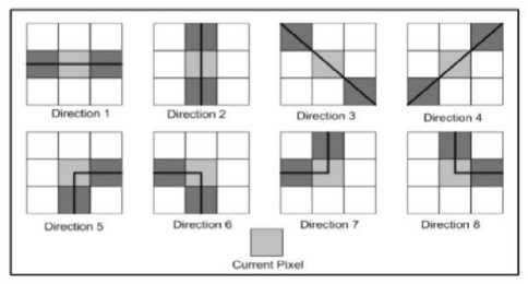
For a given way, a weighted total of the correlative components, outcomes in similar way and the weight appointed for a region is stated by:
{-1,-1… (X-1)… 1, 1}.
The similarity amid the ways (horizontal and vertical) is calculated by the following equations:
di (и,v)= -I(и-1,V)+2×I(и,V)-I(и+1,V)
d2 (и,V)= -I(и,V-1)+2×I(и,V)-I(и,V+1)
where I denotes the ultrasound image having sound (noise). Hence, the intensity-similarity estimation is by all the calculations done in all the ways. As for a specify similarity region, the intensities are immutable, thus its total is almost zero. The rate of intensity specification is given by the equation:
σ in= C× σmid (23)
Where C is a proportional factor and represents the mid of variance of M most similar regions, defined by:
σmid= ∑∑ ^ (24)
Numerator denotes the variance of the region B at (u, v) th -component. The rates of mean and variance are computed as:
∑ [X—1 ∑ jX-11 ( i , j )
μ =
w2
2 ∑ iX-1 ∑ jX-1 ( I ( i , j ) -kLuV )
ГТ — -----------------------
σ =
rate of M is estimated by the number of similarity regions having rate less than 0.5.
Relation (25) achieves the relation that shows the intensity is directly proportional to the variance (average type) of the region and thus suppresses the sound at higher level [19]. In the [20][21] (taken as example for explanation), an iterative approach is introduced to rise the presentation of Bilateral Filter. This will be an outcome in suppression of unwanted sound, with the help of SSIM [22], procured by following (successive) repetition and the stopping condition is defined by:
SSIM ( n+1 ) -SSIM ( n ) SSIM(n)
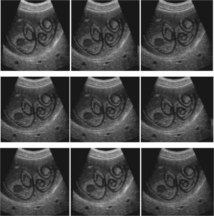
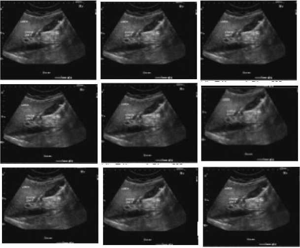
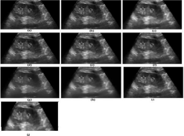
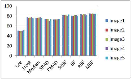
×100 Where SSIM denotes the SSIM and the above equation should be less than universal threshold and i is the ratio of the repetition. The suppression of sound is done at (i+1) th- repetition on the image procured in ith repetition and is estimated at each repetition. By the stopping criterion, the SSIM degrades as the proceeding filter. Hence, the procedure of filtering stops, in order to skip the suppression of essential information i.e. blurring of edges. F. Wavelet based bilateral filter: In [23], an approach for despeckling of an ultrasound image is proposed which is based on the wavelet thresholding and bilateral filtering. For the thresholding purpose, Neigh Shrink [24] (“thresholds the wavelet coefficients based on the magnitude of the square sum of all the wavelet coefficients within the neighborhood window”.) is consider for wavelet coefficients of the high-level detail subbands of a medical ultrasound image through wavelet filter bank during decomposition, while bilateral filtering is imposed on the approximation subband and also used after the reconstruction of an image. Thus, merging of both the steps is beneficial in preserving edges as well as in denoising and discussed one by one as follows: Wavelet thresholding: It is applied to high-level detail subbands which come from; Discrete Wavelet Transform (DWT) of an image is framed by filtering with a pair of quadrature mirror filters along both the rows and columns alternatively, depends on down sampling having a factor of 2 in every possible ways [25]. The filter procedure fragment the image into four subbands i.e. LL, LH, HL and HH. These subbands provide low frequency elements (comes in LL, in both the directions) as well as detail elements (HL, LH, HH, in horizontal, vertical and diagonal, respectively). In this transformation, small elements denote noise while large denotes necessary features of an image. The general procedure given in [23] is as follows: STEP I. Calculate the DWT. STEP II. Wavelet coefficients thresholding. STEP III. Apply inverse DWT. The wavelet coefficient is represented by: c=uf+n where u denotes noise free image and n denotes noise, uf=Sc (29) where S denotes Shrinkage factor. The threshold value is given by T, can be measured in terms of soft thresholding and hard thresholding. The function of S for Neigh Shrink for an (arbitrary 3×3) window centered at (k, l). 6-■ -=[i--h]+ (30) Where T is the universal threshold and ‘+’sign means it keeps the positive values while setting it to zero when negative and u , is the squared sum of all wavelet coefficients in the given window. - yv+1 yu+1 V2 u , = ∑ ∑ Ү , Where Y , the noisy element of estimated centre wavelet coefficient is ſ , is given by: г = 5 Y. . Bilateral filter: Already discussed in the section. Merging of wavelet thresholding and bilateral filtering: An image is decomposed into low-level (approximation) and high-level (detail subbands). Neigh Shrink is considered to threshold the coefficients of detail subband (3×3 window size and bior6.8 wavelet filter) for decomposition and reconstruction. The value of T is calculated using universal threshold [26], is stated by: T = σ√2logn (33) where σ represents standard deviation of noise and n is the signal length. The value of σ is estimated by robust median estimator [26] and is stated by: [{ , : , ∈ }] . While bilateral filtering [6] is imposed on approximation subband and after reconstruction of an image using wavelet filter bank and the parameters are estimated using multiresolution bilateral filter (related to noise standard deviation). The proposed method is given by the following diagram: Fig.2. Referred From [23] G. Multiresolution bilateral filtering: In [9], there are two main steps in this design. The first step contains the examination of the optimal parameter selection in bilateral filter and the latter contains the extension of the bilateral filter: Multiresolution bilateral filter works as, the bilateral filter is imposed on to approximation subband of an image which uses the wavelet filter bank. This design when merged with wavelet thresholding results in an effective denoising image framework, thus outcomes in eliminating noise in the given medical ultrasound image. Choice of values in bilateral filter: Both the domains (spatial and intensity) improves the behavior of the bilateral filter, but question still remains unanswered about the optimal parameter selection on theoretical basis. In [27], the nature of bilateral filter depends on derivation of given input signal and the ratio of intensity and spatial values and also discuss all the criteria on the basis of which this filter behaves like Gaussian, anisotropic and shock filters. Further, there is also an adaptive approach based on the size selection based on nonlocal neighborhood, considered as a generalized bilateral filter, produces a reduction in the local risk and the effect of intensity parameter is not taken into account [28]. Thus, the empirical study of both the parameters is necessary and considered in this section, as a function of noise variance. In [9], there are many experiments done, in order to link the standard deviations of intensity, spatial and noise. The Gaussian noise with zero-mean is used with different values of parameters, thus calculate MSE (mean squared error). The average MSE value is used to plot the analysis and observed the optimal value of spatial domain is insensitive with noise variance as compared to intensity domain. Hence, for better quality enhancement, take the range (roughly) of spatial domain and the intensity value changes significantly, as the noise variance changes its value. Multiresolution bilateral filter design: In this design, the given input signal is fragmented into subbands in terms of frequency. During reconstruction, the bilateral filter is imposed on the approximation subband which results in the reduction of low frequency noise components. This reduction is beneficial to multiresolution bilateral filter over bilateral filter [6] and this bilateral filter is of type single-level. Thus, this design concludes that the bilateral filtering is applied to approximation subband while wavelet thresholding is imposed on detail subbands, where noisy components are detected and also deleted effectively. IV. Experimental Results and Analysis In order to obtain the desired results, we compare the performance of various despeckling techniques (filters) with each other and also with three more filters namely, Lee, Frost and Median. These filters compared on ultrasound kidney and liver images with size of 257×196 pixels. We have taken PSNR (peak signal to noise ratio) parameter into account, so that we can evaluate the potency power of despeckling techniques. Fig. 3, 4 and 5, represents the filtered ultrasound images of liver and kidney, respectively. However, its corresponding performance value are measured and represented in table 1. After analyzing the manifold despeckling techniques, we can observe easily from figures, that multiresolution bilateral filter is better in reduction of speckle noise (which is taken as 0.05) among rest of the filters and also increases the enhancement quality of the ultrasound image. Multiresolution bilateral filter gives better edge preserving factor and it is observed from the figures that it have batter visual appearance in our experiments. In our experiments, the spatial adaptive filters are Lee, Frost, Median having movable window and enhance the quality of edge at some extent and estimate the statistical metrics of the pixels such as local variance and local mean. We have also taken into consideration some anisotropic diffusion filters such as SRBF, PMAD and SRAD, in which pdfs are used to directly remove the speckle noise from the ultrasound images. These anisotropic diffusion filters are having better visualization than spatial adaptive filters, due to the ability of decomposition of input signal into subbands and these subbands are despeckled and after that all of them are reconstructed, in order to provide filtered ultrasound image. Such as in case of wavelet thresholding, the decomposition of input signal is done by wavelet thresholding (produces subbands) and reconstruction of them is done by its inverse process (inverse wavelet transform). Comparison of the spatial adaptive filters i.e. Lee [29], Frost [30], and Median [31] is done after its brief description (given below). Before the description, we will show the resultant ultrasound images (3 images are used) with their visualization effects. The following ultrasound images are used to show the experimental reslts and anaylsis. These ultrasound images belongs to liver and kidneys. All the images in three figures shows: the original images , noisy image and rest of the images belongs to the filters applied on them. Fig.3. Shows, Original Image with Filtered Ultrasound Images of Liver. Fig.4. Shows, Original Image with Filtered Ultrasound Images for Kidney (With Defect) Fig.5. Shows, Original Image and Filtered Images for Kidney (Without Defect) A. Lee Filter: In [29], it is based on the MMSE (minimum mean square error), produces a noise free image given by the following equation: L(u, v) = I(u,v)F(u,v)+I’(u,v)(1-F(u,v)) (35) Where I’ denotes the mean rate of the intensity under filter and F is the collateral i.e. stated by: F (u,v) = 1- f 2 I z-2 (36) Where CN1 represents the coefficient of variation of noised image and C N represents the coefficient of variation of the noise. B. Frost filter: In [30], this filter is both adaptive as well as exponential, depends on weighted averaging filter, take the coefficient of variation which is the ratio of local standard and local mean of the image, described as below: FF = ∑ × k∝е ∝|T | (37) Where k denotes the constant,∝ is given by: ∝ =. ^,/.(σ2 /μ 2 ) (38) where σ’ is the coefficient of variance and μ represents the local mean and |T|is defined as: |T| = |X1-Xо| +|Y1-Yо | (39) And w is the size of the window. C. Median Filter: This is a nonlinear filter, removes the noise or pulse by putting the median value of its neighbors in the window in place of middle pixel value. The computation cost is its drawback having a complexity of O (N.log N) [30] [31]. We provide a median value to a particular pixel after sorting all the values in the particular window in which that pixel belongs. After examine the filtering mechanisms and compare them with the above three filters, we conclude that the output with the help of table, diagram as well as graph, shown in table1, fig 3, 4, 5 and graph1 respectively. From the results, shown in table 1 (mentioned below), the PSNR value of the multiresolution bilateral filter is larger than all other filters (considered). Thus, this filter observed as the most suitable speckle reduction technique among others. The PSNR is however, calculated by the following formulation: PSNR=10log10 ( ) (40) MSE= й×у∑i=l ∑j=l (x i,j -yi,j)2 (41) Where MSE denotes Mean Square Error, U×V is the size of the window and x, y denote the original as well as denoised images. We used MATLAB R2009a to evaluate the result and experiment the despeckling techniques on more than 5 ultrasound images on various human organs and showing the result of 5 images and visualization of 3 ultrasound images in this review paper. In the experiment, we focus on the performance metric and edge enhancement. The images for all the filters are given. These images of ultrasound are for liver (fig. 3), for kidney with defect (fig. 4) and for kidney without defect (fig. 5) are discussed above. Now the PSNR value for all the filters, calculated from the images obtained after applying the mechanisms are shown in the below table i.e. Table 1. Table 1.shows the results of various filters using PSNR parameter Images/ filters Image1 Image2 Image3 Image4 Image5 Lee 50.77 77.41 76.27 74.27 73.01 Forst 49.67 76.4 76.10 73.56 72.95 Median 50.11 76.78 77.01 74.13 73.24 SRAD 50.46 77.56 77.34 70.24 74.01 PMAD 51.34 75.78 76.20 73.48 73.98 BF 50.77 77.41 76.27 74.27 73.01 ABF 49.67 76.4 76.10 73.56 72.95 MBF 50.11 76.78 77.01 74.13 73.24 And finally we plot a graph i.e. Graph 1(shown below) for the PSNR values, in order to visual our result, more effectively. Graph 1 shows comparison between filters and PSNR value V. Conclusion and Fututre Aspects In this paper, we make a survey on the PSNR value of manifold filters in image denoising applications. As we observed that speckle filters results in case of ultrasound medical images, but have some drawbacks which outcomes in resolution degradation. The filters are adaptive as well as non-linear. It is examined that adaptive filters results in similar visual appearance while non-linear filters results in high performance with better appearance. Furthermore, the multiresolution bilateral filter, which is a merger of bilateral filter and wavelet thresholding due to its multiresolution application, exhibits high performance and ability to preserve and enhance the edges in among all the despeckling techniques in ultrasound medical image. The enhancement property in also there in adaptive like SRBF, but due to thresholding concept, it enhance more in multiresolution bilateral filter. We used a specific technique for wavelet thresholding (BayesShrink method). As multiresolution bilateral filter helps in removing noise from the images and results better due to wavelet thresholding, which remove noise components in detail subband more efficiently. We can also use different wavelet thresholding techniques for comparison. After comparing the PSNR value on more than 50 ultrasound medical images, we conclude that multiresolution bilateral filter provides better performance among the rest of the filters. The other parameters comparison is referred as future work, in which we can take SSIM, SNR, AD, SI and EPF.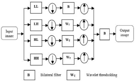
Список литературы Despeckling of Medical Ultrasound Images: A Technical Review
- Goodman, Joseph W. "Statistical properties of laser speckle patterns." Laser speckle and related phenomena. Springer Berlin Heidelberg, 1975. 9-75.
- F.Wagner, S.W. Smith, J.M.Sandrik, and H. Lopez, "Statistics of speckle in ultrasound B-scans," IEEE Trans. Sonics Ultrason., vol. 30, pp. 156–163, May 1983.
- Sehgal, "Quantitative relationship between tissue composition and scattering o of ultrasound," J. Acoust. Soc. Amer., vol. 94, pp. 1944–1952, Oct. 1993.
- T.Loupas, W. N. McDicken, and P. L. Allan, "An adaptive weighted median filtlaser for speckle suppression in medical ultrasound images," IEEE Trans. Circuits Syst., vol. 36, pp. 129–135, Jan. 1989.
- M. Karaman, M. A. Kutay, and G. Bozdagi, "An adaptive speckle suppression filter for medical ultrasound imaging," IEEE Trans. Med. Imag., vol. 14, pp. 283–292, June 1995.
- C. Tomasi and R. Manduchi, "Bilateral filtering for gray And color images", in IEEE International Conference on Computer Vision, pp.839–846, 1998.
- Farzana, E., et al. "Adaptive bilateral filtering for despeckling of medical ultrasound images." TENCON 2010-2010 IEEE Region 10 Conference, IEEE, 2010.
- B. Zhang and J. P. Allebach "Adaptive bilateral filter for sharpness enhancement and noise removal", IEEE Trans. Image Process., vol. 17, no. 5, pp.664 -678 2008
- M. Zhang and B. K. Gunturk "Multiresolution bilateral filtering for image denoising", IEEE Trans. Image Process., vol. 17, no. 12, pp.2324 -2333 2008.
- A. K. Jain, Fundamental of Digital Image Processing. Englewood Cliffs, NJ: Prentice-Hall, 1989.
- X. Zong, A. F. Laine, and E. A. Geiser, "Speckle reduction and contrast enhancement of echocardiograms via multiscale nonlinear processing," IEEE Trans. Med. Imag., vol. 17, pp. 532–540, Aug. 1998.
- A. Achim, A. Bezerianos, and P. Tsakalides, "Novel Bayesian multiscale method for speckle removal in medical ultrasound images," IEEE Trans. Med. Imag., vol. 20, pp. 772–783, Aug. 2001.
- M. Tur, K. C. Chin, and J. W. Goodman, "When is speckle noise multiplicative?," Applied Optics, vol. 21, pp. 1157–1159, Apr. 1982.
- Jadwiga Rogowska and Mark E. Brezinski, "Evaluation of the adaptive speckle suppression filter for coronary optical coherence tomography imaging," IEEE Transactions on Medical Imageing, Vol. 19, No. 12, pp. 1261–1266, 2000.
- Yongjian Yu and Scott T. Acton, "Speckle reducing anisotropic diffusion," IEEE Transactions on Image Processing, Vol. 11, No. 11, pp. 1260–1270,2002.
- Joachim Weickert, "Anisotropic diffusion in image processing,"B.G. Teubner (Stuttgart), pp. 14–29, 1998.
- Simone Balocco, Carlo Gatta, Oriol Pajol, Josepa Mauri, and Petia Radeva, "SRBF: Speckle reducing bilateral filtering," Ultrasound in Medical & Biology, Vol. 36, No. 8, pp. 1353–1363, 2010.
- G. Wyszecki and W. S. Styles. Color Science: Concepts andMeth- . ods, Quantitative Data and Formulae. Wiley, New York, NY, 1982.
- A. Amer and E. Dubois, "Fast and reliable structure-oriented video noise estimation", in IEEE Trans. on Circuits and Systems for Video Technology, vol. 15, no. 1, pp. 113–118, 2005.
- M. Elad, "On the origin of the bilateral filter and the ways to improve it", in IEEE Trans. on Image Process., vol. 11, no.10, pp. 1141–1151, October, 2002.
- D. Barash, "Fundamental relationship between bilateral filtering, adaptive smoothing, and the nonlinear diffusion equation", in IEEE Transactions on Pattern Analysis and Machine Intelligence, vol. 24, no. 6, pp. 844–847, 2002.
- Z. Wang, A. C. Bovik, H. R. Sheikh and E. P. Simoncelli,"Image quality assessment: from error visibility to structural similarity", in IEEE Trans. on Image Process., vol. 13, no. 4, pp. 600–612, April, 2004.
- R.Vanithamani and G.Umamaheswari "Wavelet based Despeckling of Medical Ultrasound Images with Bilateral filter", 2011, 389-393.
- G.Y.Chen,T.D.Bui and A.Krzyzak, "Image denoising using neighbouring wavelet coefficients" 2004,ICASSP, IEEE, pp. 917-920.
- S.Mallat, A theory for multiresolution signal decomposition: The wavelet representation, IEEE Trans. Patterns Anal. Machine Intell. 11 (1989) 674– 692.
- D.L. Donoho, I.M. Johnstone, "Ideal Spatial Adaptation via Wavelet Shrinkage", Biometrika, vol.81, pp.425~455, 1994.
- A. Buades, B. Coll, and J. Morel, "Neighborhood filters and PDE's," Numer. Math.,vol. 105, pp. 1–34, 2006.
- C. Kervrann and J. Boulanger, "Optimal spatial adaptation for patchbased image denoising," IEEE Trans. Image Process., vol. 15, no. 10, pp. 2866–2878, Oct. 2006.
- R. Sivakumar, M. K. Gayathri and D. Nedumaran, "Speckle filtering of Ultrasound B-scan images - A comparative study between spatial and diffusion filters," 2010 IEEE Conference on Open System (ICOS 2010), pp. 80-85, 2010.
- RamanMaini, Himanshu Aggarwal, "Performance evaluation of various speckle noise reduction filters on medical images," International Journal of Recent Trends in Engineering. Vol. 2, No. 4, pp. 22-25, 2009.
- Jadwiga Rogowska and Mark E. Brezinski, "Evaluation of the adaptive speckle suppression filter for coronary optical coherence tomography imaging," IEEE Transactions on Medical Imageing, Vol. 19, No. 12, pp. 1261-1266, 2000.
