Detecting Android Malware by Mining Enhanced System Call Graphs

Today, Android is the most widely used mobile operating system. There is 86 percent of smartphones use Android as the operating system [1]. The challenges also followed its popularity, including negative ones like malware. Attacks caused by malware cause various kinds of damage. They start with minor inconveniences such as making the smartphone heavier, displaying random advertisements, downloading additional code, etc. The malware can cause serious damage, such as data theft, extortion, spying, and device hijacking. Meanwhile, thousands of new malware appear every day [2]. Android is the target of up to 98 percent of mobile malware [3].

Malware detection reduces the impact of malware assaults. In the detection procedure, signature-based detection employed a known pattern. The benefit of this detection method is that it is efficient and produces few false alarms. Signature-based detection, on the other hand, has a number of drawbacks, including the inability to identify new or undiscovered malware and the need to update the database regularly [4]. Contrary, Heuristic-based detection can detect unknown malware. It employs sophisticated methods to identify harmful software, such as a rule-based system or machine learning utilized in the process [5].

The heuristic technique relies on retrieving several features from the malware as part of the detection process. Retrieving the features can be accomplished dynamically or statically. Static analysis is done by analyzing the Android APK file. The process starts with unpacking the Android APK file and observing the items contained. Some of the features that result from the static analysis are permissions, intent filters, API calls, etc. [6]. Static analysis is limited because of its inability to process native and obfuscated codes [7].

Dynamic analysis can overcome the weakness of static analysis mentioned above [8]. The application features may emerge due to its execution in a predetermined environment, then monitoring the activity and behavior of the application being executed. Some of the features that can be taken from the dynamic analysis include system calls, network activity, CPU usage, memory usage, etc. [6].

In this paper, we will be focusing on the system calls of an application and using them as our detection features. A system call is an intermediary between the program and the Linux kernel [9]. Like other operating systems, Android enforces abstractions so that apps require system calls to get a service from the kernel. Thus, the behavior of an Android application can be recognized from a sequence of system calls that manifest. For example, making connections, writing files, executing threads, etc.

A series of certain system calls can be considered suspicious activity if they come out of things that are deemed normal from an application. For example, an Android application attempts to gain elevated access to the system by repeatedly accessing core system files. This could indicate malicious behavior, as legitimate applications typically do not need to repeatedly access these types of files. The repeated attempts to access the files may be an attempt to exploit vulnerabilities in the system or bypass security measures, allowing the application to perform unauthorized actions.

Graphs are a useful tool for representing malicious behavior because they can illustrate how different entities in a system interact in unusual or suspicious ways [10]. In this context, a graph consists of nodes representing system calls and edges representing the control flow between them. By analyzing the graph, it is possible to identify behavior patterns indicative of malware. Furthermore, machine learning algorithms can be trained to study these patterns and classify them into benign and malicious behaviors.

Therefore, this study will analyze the use of graphs in Android malware detection. Feature selection involves identifying the most relevant and informative features of a dataset and using them to build a predictive model.

The contributions of this paper are listed as follows:

• •    Describe the various types of system call representations that are used as material input in the detection of Android malware, including the strengths and weaknesses of each.

• •    Propose a graph-based processing and representation of system calls in order to minimize the loss of valuable information.

• •    Proposed a detection architecture based on the system call graph.

• •    Propose a series of feature selection methods to improve detection accuracy.

• •    Use the most up-to-date malware data set to evaluate our detection architecture.

2.    Recent Works

The structure of this paper can be described as follows: In Section II, we discuss the recent works and the types of system call representations that are used as detection material. Each type of feature representation has certain characteristics that can affect the detection results. Section III describes our research methods, including the dynamic analysis, generating and processing of the features, and the detection system. We explain the implementation scheme in Section IV, as well as the dataset, environment setup, and evaluation procedure. In Section V, we show the result of feature selection and classification. In Section VI, we examine our findings and draw some conclusions. Finally, we give suggestions for future research in Section VII.

A number of studies have been carried out on the Android operating system to investigate the identification of malicious code. In this paper, research related to system calls as detection material, either as a stand-alone feature or in combination with other features, will be divided into several groups based on how they are processed, namely: as histogram, TF/IDF, N-gram, Markov chain, others.

TF/IDF is a statistical method used to understand how important a word is to a document or a corpus [11]. This technique calculates Term Frequency (TF) and Inverse Document Frequency (IDF) values for all words in a document. The TF-IDF technique determines how frequently a word appears in a document. In the context of malware analysis, it relates to how often a system call function occurs. Several studies use TF/IDF as feature representation, namely Deepa et al. [12], Nguyen et al. [13], and Das et al. [14]. However, this method may lose information from the sequence of system call operations. The presence of system calls in chronological order could indicate malicious behavior. In this situation, the nature of TF/IDF, which calculates weights per word occurrence, cannot accurately depict malicious behavior.

In another study, Chaba et al. [15] used a technique that records the presence of a given function in a system call sequence. If a function appears in a system call sequence, the occurrence of that function is assigned a value of 1. Whereas if it does not appear, the occurrence of that function is assigned a value of 0. We believe that the binary occurrence representation is inaccurate as it causes a lot of information to be lost, for instance, the order and frequency of occurrences.

Markov chain is a sequence of events in which the conditional probability of future events depends on the current events. In the context of malware detection, Ahsan-Ul-Haque et.al. [23], Xiao et al. [24] use Markov chains to extract the characteristic of malicious behavior from its system call sequences. Through this approach, sequences can be maintained. However, Markov models are thought to be troublesome at small time periods [25].

The co-occurrence matrix is usually used to measure texture in the field of image processing. Some literature such as Xiao et al. [26], Borek et.al [27], Thuan et.al. [28], Xiao et al. [29], Wang et al. [30] use co-occurrence matrix in malware detection problem. It is calculated by counting the number of transitions from point to point in k distance. Thus, each element of the co-occurrence matrix shows the intensity of the correlation between two points within a certain distance. This method can keep the relation between system calls. However, at distances k > 2, it may be less significant since the information in the co-occurrence matrix will be less precise if a function runs on a different thread. If the function runs on a different thread, then the context is different.

The studies mentioned above have weaknesses in terms of the representation of the system call as a feature. A mistake in feature representation might lead to the loss of important information and impact the quality of malware detection. Therefore, in this paper, we propose a representation of the system call in the form of a graph. As a result, important information, such as the appearance of a function and the order of system calls, is thought to be preserved. Machine learning is expected to improve detection results.

3.    Proposed Method

The design of a malware detection system is a complex process that involves several stages. One of the main stages is dynamic analysis, which involves observing the behavior of a malware sample as it executes in a controlled environment to identify its malicious activities. The second stage is featuring processing, which involves extracting relevant features from the dynamic analysis data and converting them into a format that can be used by the classification engine. Finally, the classification engine uses machine learning algorithms to analyze the feature data and determine whether the sample is malicious or benign. These three stages are essential in designing an effective malware detection system. Fig.1 p rovides an overview of the main design of a malware detection system. The details of each stage will be explained in their respective subsections.

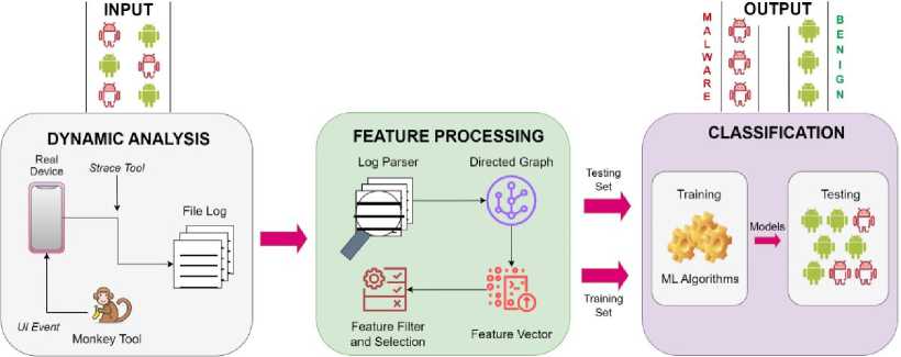
Fig.1. Overview of the main design of a malware detection system

• 3.1.    Dynamic Analysis

This stage aims to monitor the behavior of applications that are executed in a controlled environment and then save the behavior in a log file. The APK files of these applications are loaded into real mobile devices. A system call sequence is used to describe the behavior of a running application. A system call is an intermediary facility when an application requests services from the OS kernel, such as establishing an Internet connection or transferring data. Thus, in this method, the behavior of an application is characterized by the usage of system calls.

System call, as a characteristic of application behavior, is triggered if the application gets an external stimulus, such as user interactions. For example, the touch, double-tap, swipe, scroll, and other UI events may be used to create these interactions. There are automated technologies that mimic human behavior, such as Monkey tools, which can be used to substitute user involvement. In this paper, we use 1,000 automated random UI events to simulate user interactions with the applications.

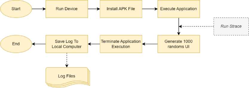
Fig.2. The execution of malware during dynamic analysis

By monitoring the system calls made by a running application, it is possible to identify any anomalous behavior that could indicate the presence of malware. The process involves hooking the application's system call interface to intercept and log all system calls made during execution, which are then saved to a log file for further analysis. To achieve this, we use the process described in fig.2 and follow the steps outlined below:

• •    Run the real device.

• •    Install the APK file of the application on the real device.

• •    Execute the application on the device and obtain the package name of the application.

• •    Get the package-matching zygote PID, then start recording the system calls using the strace command.

• •    Generate 1000 random UI events using Monkey tools.

• •    Terminate application execution in the device.

• •    Copy the system call logs using the adb pull command.

The log file generated from observing the application in the device environment contains system calls that are chronologically sequential from the start of the application execution until it is terminated. In each line of the logs file, the name of the call function, input values, and return value are listed. System calls that are ordered chronologically can help us understand how an application works when it is run. Fig.3 depicts an example of the log file containing system call lines.

clock_gettime (CLOCK_MOKOTONIC, {37665, 454801500}) = 0

epoll_pwait(27, [], 16, 253, NULL, 8) = 0

clockgettime(CLOCKMONOTONIC, {37665, 712682800}) =0

clock_gettime(CLOCK_MONOTONIC, {37665, 714343400}) =0

clock_gettime(CLOCK_MONOTONIC, {37665, 715887900}) =0

recvfrom(35, 0xbf88f9c8, 2400, MSG_DONTWAIT, NULL, NULL) = -1 EAGAIN (Try again)

clock_gettime(CLOCK_MONOTONIC, {37665, 720415700}) =0

clock_gettime(CLOCK_MONOTONIC, {37665, 721477400}) =0

epoll_pwait(27, [], 16, 0, NULL, 8) = I clockgettime(CLOCKMONOTONIC, {37665, 721843000}) = 0

epoll_pwait(27, [{EPOLLIN, {u32=35, u64=35}}], 16, -1, NULL, 8) = 1

recvfrom(35, ”nysv\0\0\0\0#m\211\274A\,T\0\0%\36\0\0eate", 2400, MSG_DONTWAIT, NULL, NULL) = 2^

recvfrom(35, 0xbf88fcl8, 2400, MSG_DONTWAIT, NULL, NULL) = -1 EAGAIN (Try again) clock_gettime(CLOCK_MONOTONIC, {37665, 719464500}) =

Fig.3. System call sequence in the log file

• 3.2.    Feature Processing

The objective of this stage is to parse relevant information from the log files and convert them into feature vectors that can be utilized as input for the classification engine. The process begins with loading the log files and reading their contents. The next step is to identify the system calls that exist in the log files and calculate and plan the graph that will be built. To simplify the process, this research represents the graph in a adjacency matrix. The final step in this stage is to transform the adjacency matrix into a feature vector that can be used as input for the classification engine. This stage is critical for the success of the malware detection system as it transforms the raw data into a format that can be easily understood and processed by the classification engine. fig.4 provides a summary of the proceses performed during this stage.

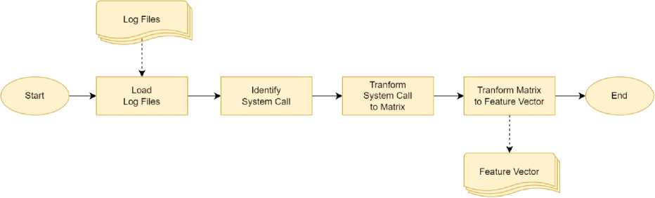
Fig.4. The process involves parsing log files and transforming them into a feature vector

To read system call in a log files, formally, we can define S = {s 1 , s₂, .., s _n } as the set of all function names of all system calls contained in an Android operating system. While the sequence of system calls along m in the chronologically arranged log file can be defined as Q = {q 1 , q₂,...., q_m], whereq ; E S is the contents of the log file on line i. In addition, to call sequences, the application can use the clone() or fork() functions to operate several threads, which allows for numerous branching in system call execution. In such cases, the execution of the system call can be represented as a graph. Fig.5 illustrates an example of a sequencing system calls as a graph.

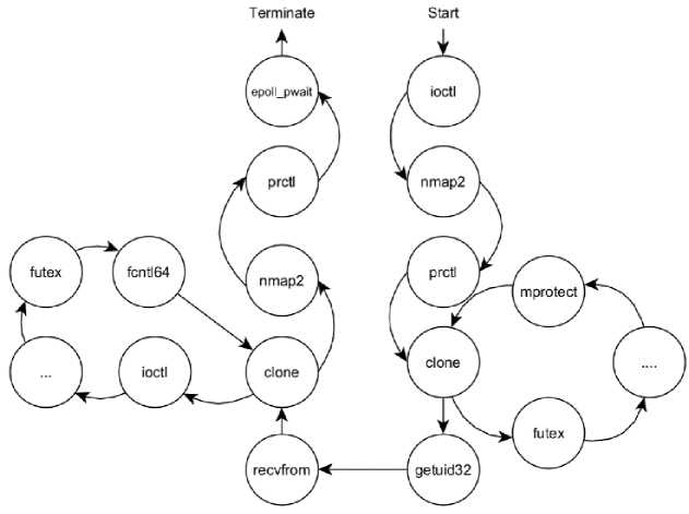
Fig.5. An example of a graph representation of a system call sequence

Denote G = (V,E) as a graph with V as vertex or node and E as edge or direction; each node V corresponds to one line of a system call that appeared in the log file. If и and v EV, then (u, v) E E is the direct link from one node to another node. For each logged system call of the monitoring application, we describe the relationship between system calls as an adjacency matrix containing the number of occurrences of potential transitions from и to v.

Table 1. Example of graph transition of a system call in the form of the adjacency matrix

	clock_gettime	epoll_wait	recvfrom
clock_gettime	3	3	1
epoll_wait	2	0	1
recvfrom	2	0	1

The chronological appearance of system calls, as illustrated in Fig.3, might be transformed into an adjacency matrix containing the transition from one system call to another. In Table 1, the transition graph was presented in the form of a 3x3 adjacency matrix. The value of the adjacency matrix is calculated from the transition between system calls. For instance, the transition from clock_gettime to epoll_wait occurs three times; therefore, the transition value in the matrix is 3. In the same way, the transition from recvfrom to clock_gettime occurs twice, so the value of the matrix transition is 2. Meanwhile, the transition from recvfrom to epoll_wait never occurs; therefore, the matrix transition value is 0.

In this paper, we considered 282 system calls based on the version of Android 11, with 11 additional system calls provided to accommodate a lower version of Android. This is different from Xiao et al. [24] study, in which they used 196 system calls, while Xu et al. used 213 system calls [31]. Some other studies did not pay attention to how many system calls are used.

Algorithm 1 . Transform a system call graph into an adjacency matrix and feature vector.

1	public syscall_x, syscall_y, syscall_matrix, feature_vector
2
3	Function IdentifySystemCall(File LogFile){
4	# initializing index name for system call
5	this.syscall_x ← new Array()
6	this.syscall_y ← new Array()
7
8	# read log file line by line
9	content ← file_get_contents(LogFile)
10	:      lines ← new Array(explode("\n", content))
11
12	:     # find all of the system call names from one log file
13	:      for i ← 0 to count(lines) - 2 do
14	:       # find the system call name of 1st node
15	:       syscall_name ← FindSystemCallName(lines[i])
16	:       this.syscall_x[syscall_name] ← NULL
17
18	:       # find the system call name of 2nd node
19	:       syscall_name ← FindSystemCallName(lines[i]+1)
20	:       this.syscall_y[syscall_name] ← NULL
21	:      endfor
22	:         }
23	:   Function SystemCallGraph2Matrix(File LogFile){
24	:     # represent system call graph in the form of array 2d / matrix
25	:     # the number of matrix elements = count(this.syscall_x) * count(this.syscall_y)
26	:     # assign each element of the matrix with a zero value
27	:     this.syscall_matrix[count(this.syscall_x)][count(this.syscall_y)] ← new Array() * 0
28
29	:      # read log file line by line
30	:      content ← file_get_contents(LogFile)
31	:      lines ← new Array(explode("\n", content))
32
33	:      # for each line of the log file record system call transition
34	:      for i ← 0 to count(lines) - 2 do
35	:       # find the system call name of 1st node
36	:       x ← FindSystemCallName(lines[i])
37	:       # find the system call name of 2nd node
38	:       y ← FindSystemCallName(lines[i]+1)
39	:        # record system call transition from node x to y (1st to 2nd node)
40	:        this.syscall_matrix[x][y]++
41	:      endfor
42	:         }
43	:   Function Matrix2FeatureVector(){
44	:      i ← 0
45	:     # create an empty feature vector in a temporary variable
46	:     tmp ← new Array()
47
48	:     # transform from system call matrix to feature vector
49	:      foreach this.syscall_x as key_x => val_x do
50	:        foreach this.syscall_y as key_y => val_y do
51	:          tmp[i] ← this.syscall_matrix[key_x][key_y]
52	:            i++
53	:        endforeach
54	:      endforeach
55	:     # save feature vector to single string separate by commas
56	:     this.feature_vector ← new Array(implode(",", tmp))
57	:         }

The probability of transition from и to v can be accommodated in a matrix with 282x282 dimensions. However, not all system calls are used during the execution of an application. To reduce the computational cost, we only record the system calls that appear during the execution of the application. This allows us to focus on the most relevant system calls and improve the efficiency of the analysis.

The final task of feature processing is transforming the adjacency matrix to the feature vector, called vectorization. Denote Vec(A) with mn x 1 column is the transformation of matrix A with mxn column by stacking rows in matrix A on top of each other. Algorithm 1 describes the generation algorithm of the system call sequence to the adjacency matrix and then transforms it into a feature vector. While Table 2 depicts the result of the transformation from the adjacency matrix into a feature vector. The transformation is based on the example data represented on the matrix from Table 1.

Table 2. Example of feature vector transformation from the adjacency matrix

clock_ gettime x clock_ gettime	clock_ gettime x epoll_ wait	clock_ gettime x recvfrom	epoll_ wait x clock_ gettime	epoll_ wait x epoll_ wait	epoll_ wait x recvfrom	recvfrom x clock_ gettime	recvfrom x epoll_ wait	recvfrom x recvfrom
3	3	1	2	0	1	2	0	1

• 3.3.    Feature Filter and Feature Selection

• 3.4.    Classification

• 3.5.    Real Device Setup

Before being fed to the classification engine, the feature vector needs to be improved. This stage aims to select features that have a significant impact on the classification process. In other words, feature selection can help improve classification results. In this paper, we applied two filters. First, we remove useless features with zero value. Second, we use the Gain Ratio feature selection algorithm. This algorithm is considered an improvement over the Information Gain algorithm because it reduces bias [32]. The Gain Ratio is frequently used to identify numeric (continuous) and categorical or discrete characteristics. The Gain Ratio technique is a justifiable choice because the attribute used in this study is a continuous attribute type. The detailed process of feature filtering and feature selection can be seen in fig.6.

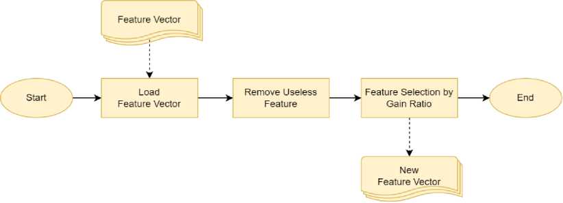
Fig.6. Feature filter and feature selection process

This stage aims to classify the data as either malware or benign. Classification is a grouping of data where the data used has a label or a target class. In predictive modeling, classification is used to assign a class label to input data. Classification engines can be employed to detect malicious behavior by identifying patterns that arise from a sequence of system calls. To achieve this, the classification engine uses various algorithms to build models based on the feature vectors obtained in the previous stage. Among them are: AdaBoost, Decision Table, Naïve Bayes, Random Forest, IBk, J48, and Logistic regression.

In order to ensure the best performance and generalization ability of the models, a 10-fold cross-validation technique is utilized to test each model. This involves dividing the data into 10 equal parts, with each part being used as a testing set once and the remaining 9 parts used as training sets to train the model. This process is repeated 10 times so that each part is used as the testing set once.

Each malware application is executed on a real device to obtain the system call. Using real devices helps circumvent anti-emulation techniques, as mentioned in [33]. Furthermore, utilizing real devices enables the simulation of real-world smartphone functionality. For instance, to serve as a communication tool, a smartphone requires a SIM card for communication over cellular networks, as well as an internet connection for communication with the outside world through the internet. The configurations specified in Table 3 are expected to provide optimal detection results by closely resembling real-world scenarios.

Table 3. The setting of the device environment

No.	Configuration	Status
1	SIM card	Inserted, active
2	Cellular network	Active
4	Airplane mode	Off
5	WiFi	Yes
6	Data connection	Off
7	Internet connection	Yes, through WiFi
8	Phone contact	Present
9	SMS Inbox	Present
10	Call history	Present

4.    Implementation

In this section, we will go over to implement the method that was proposed in the previous section. In addition, this section describes the dataset that will be utilized, how to build the environment, and how to evaluate the results of the Implementation.

• 4.1.    Data set

  This study uses a publicly available data set called MalDroid-2020 [34]. The data set contains a thousand samples of Android malware and benign applications in the form of APK files. We select the data set by applying some criteria as follows,

  • •    We choose only the applications with an Android OS version above 5.0, codename Lollipop. We did so because we wanted to select a data set that resembles the population of Android versions on the market [35].

  • •    We chose a balanced dataset of 4064 applications, consisting of 2032 malware and 2032 benign samples.

• 4.2.    Experimental Setup

• 4.3.    Evaluation

In our experiment, we perform dynamic analysis on sixteen real devices, including SM-J120, SM-J111, SM-G532, and SM-J330. The devices are arranged according to the configuration specified i n Table 3 t o mimic real-world conditions as closely as possible. Table 4 shows the detailed configuration of the real device along with the application data set. For classification purposes, we use Weka software version 3.5.9 [36]. We employ a small PHP script to transform the system calls into a matrix. The matrix is then transformed to feature vector mode. The transformation process is based on Algorithm 1.

Table 4. The configuration of devices along with application in the data set

No.	Device	Number of Analyzed Applications	Type of Application	No.	Device	Number of Analyzed Applications	Type of Application
1	SM-J120	160	Malware	6	SM-J120	123	Benign
2	SM-J111	1153	Malware	7	SM-J111	965	Benign
4	SM-G532	695	Malware	8	SM-G532	716	Benign
5	SM-J330	24	Malware	9	SM-J330	228	Benign
Total		2032	Malware	Total		2032	Benign

This stage explains the methodology to evaluate the performance of the proposed method. We use a 10-fold crossvalidation technique to test each classification model in order to get the best model with the best generalization ability. The data set is split into ten equal subsets, with 90% of the instances used to construct the training model and 10% used as a test set. The confusion matrix shows the number of samples that were correctly or incorrectly classified, as shown in Table 5.

Table 5. Confusion matrix

	Target Positive	Target Negative
System Positive	True positive ( t p )	False positive ( f p )
System negative	False negative ( f n )	True negative ( t n )

The confusion matrix can be used to determine several metrics for measuring the effectiveness of a malware detection system, such as:

• •    Accuracy. The accuracy is computed by dividing the number of samples for which the prediction was accurate by the total number of samples. It indicates the percentage of accurate predictions provided by the detection engine.

  Accuracy =

  
  

  tp + tn

  tp + fp + tn + ft

  
  
  
  

• •    Precision. The precision of a detection system is calculated by dividing the number of accurately recognized positive samples by the total number of samples anticipated as positive. It indicates the proportion of projected positive samples that were accurate.

  Precision =

  
  

  t_p

  tp + f_P

  
  
  
  

• •    Recall. The proportion of positive samples that were accurately predicted is divided by the total number of true positive samples. It assesses a classifier's ability to correctly identify samples belonging to a particular class.

  Recall =

  
  

  t_p

  tp + f_n

  
  
  
  

• •    False Positive Rate (FPR). The rate of false positive predictions is determined by dividing the total number of inaccurate positive predictions by the total number of true negative cases. FPR is utilized to determine the probability of a false alarm.

  FPR =

  
  

  fp

  
  

  fp + tn

  
  
  
  
5.    Experimental Result

The Android application is executed in a real device environment. A series of system calls could represent malicious behavior. A system call can be associated as a feature. The system calls are extracted using the strace tool and then transformed into the form of a feature vector, as explained in Section III. In this section, the experiment is conducted by following the two schemas shown below:

• •    The Implementation and result of feature processing.

• •    The Implementation and result of the feature selection methodology.

• •    The Implementation and result of numerous machine learning algorithms.

• 5.1.    The Implementation Feature Processing

  In this schema, each Android application in the MalDroid-2020 data set is executed on a real device. It allows us to analyze the activity of malware by monitoring the system calls made during its execution. The probability of system call transformation is 282x282 of matrix dimensions. It will generate a feature vector with 79,524 features. However, as mentioned in Section 3.B, we recognize that not all system calls are used during the execution of an application; therefore, to minimize computation cost, we only record the system calls that are actually used. Based on the vectorization algorithm outlined in Algorithm 1, a vector that contains a total of 28,224 features is produced. Table 7 shows feature processing results with reduction percentages.

• 5.2.    Feature Selection Implementation and Result

Table 6. The reduction of the feature vector is achieved by selecting only the system calls that were used during execution

	Number of Features	Reduction Percentages
Probability of feature 282x282	79,524	-
The actual feature produced with the removal of unused system call	28,224	64.50%

In the feature processing stage, we produce 28,224 features. However, that is a significant amount for a feature. Therefore, the feature selection process provided in section 3 .0 is required. The feature selection order is to eliminate useless features, then implement the Gain ratio algorithm. The phases of the feature selection process are depicted in

Table 7, along with the outcomes of each stage. This demonstrates that the proposed feature selection process may eliminate features by as much as 91.95%. While Table 8 shows the top 20 features ranked using gain ratio and the number of system call occurrences on benign and malware.

Table 7. The Implementation of the feature selection method

	Number of Features	Reduction Percentages
Original Features	28,224	-
Remove Useless	3,542	87.45%
Gain Ratio	2,270	91.95%

Table 8. The top 20 features rank using the gain ratio

No	Feature	Number of Occurrences		Gain Ratio Score	No	Feature	Number of Occurrences		Gain Ratio Score
		Benign	Malware				Benign	Malware
1	fstat64_fchmodat	8,955	125	0.29516	11	setsockopt_getsockopt	4,992	484	0.23713
2	clock_gettime_ftruncate64	2,6223	4,552	0.27186	12	rt_sigreturn_connect	2	477	0.22904
3	fsync__llseek	2,984	14	0.26762	13	fstat64_gettimeofday	7,908	1,078	0.218
4	pselect6_setsockopt	3,290	3	0.26689	14	gettid_close	19,331	126,731	0.21395
5	_llseek_fsync	2,270	8	0.26395	15	mmap2_gettid	24,126	160,534	0.2139
6	fchmodat_write	5,929	134	0.24394	16	newfstatat_fchmodat	3,492	63	0.21277
7	mlock_munlock	2,219	31	0.24128	17	gettid_munmap	743	19,804	0.21234
8	mmap2_mlock	2,204	32	0.23977	18	futex_rt_sigtimedwait	54	1,057	0.20997
9	munlock_openat	1,111	16	0.23952	19	getuid32_faccessat	5,064	304	0.20953
10	munlock_getsockopt	1,029	16	0.23851	20	sigaction_mprotect	1,551	5,591	0.20948

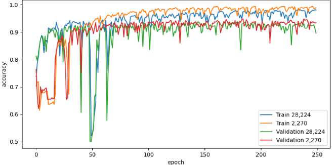
Fig.7. The impact of applying feature selection on the model accuracy

Fig.7 depicts a comparison when applying the classification model to a kind of data set, i.e., before and after feature selection, with a number of features of 28,224 to 2,270, respectively. The observations showed that reducing the number of features could improve the accuracy of the classification model. It indicates that our selection method provides better detection results.

• 5.3.    Classification Result

This section discusses the classification process through numerous machine learning algorithms, i.e., AdaBoost, Decision Table, Naïve Bayes, Random Forest, IBk, J48, and Logistic regression. We use the ten k-fold cross-validation method to assess the classification performance. The classification uses a filtered data set resulting from the previous process through feature selection.

Table 9 shows the classification results using various machine learning algorithms and evaluation metrics. These benefits are dispersed equitably among all machine learning methods. The best results were obtained by the Random Forest classification and followed by another classifier. At the same time, the Naive Bayes algorithm demonstrates the highest accuracy in identifying malicious applications.

Table 9. Classification using numerous machine learning algorithms

Classifier	Sample Category (%)	FPR (%)	Prec. (%)	Rec. (%)	Acc. (%)	Acc. Total (%)
Adaboost	Benign	8.5	91.2	87.9	87.89	89.69
	Malware	12.1	88.3	91.5	91.49
Decision Table	Benign	10.7	89.4	90.4	90.35	89.81
	Malware	9.6	90.2	89.3	89.27
Naïve Bayes	Benign	8.0	90.8	79.6	79.63	85.80
	Malware	20.4	81.9	92.0	91.98
Random Forest	Benign	5.40	94.7	96.1	96.06	95.32
	Malware	3.90	96.0	94.6	94.59
IBk	Benign	5.4	94.2	87.1	87.06	90.84
	Malware	12.9	88.0	94.6	94.64
J48	Benign	7.0	92.9	91.1	91.14	92.07
	Malware	8.9	91.3	93.0	93.01
Logistic Regression	Benign	6.2	93.3	86.3	86.32	90.08
	Malware	13.7	87.3	93.8	93.85

In this study, we further evaluate the proposed method using well-known antivirus programs that are already on the market. Some of these are Avira, Kaspersky, Avast, Symantec, Comodo, ClamAV, BitDefender, and F-Secure. For this purpose, we examined malicious applications on the MalDroid-2020 data set to be compared. Antivirus app scan facility provide through VirusTotal API. The statistics depicted in fig.8 shows that our proposed system gives equal or even better detection result than several existing antiviruses.

Fig.8 also highlights that antivirus software like Avira and Kaspersky may offer slightly better detection results. However, they may become ineffective in detecting malware that uses defense mechanisms like obfuscation. This is because the detection method that relies on MD5/SHA1 hash signatures database can be easily fooled by obfuscation, as revealed by the Preda&Maggi study [37]. On the other hand, the proposed method in this study employs dynamic analysis, which is more resilient to obfuscation and can detect even the most advanced malware.

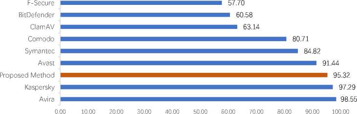
Fig.8. The comparison of detection results between our detection model and existing antivirus software

6. Conclusions

The state-of-the-art of utilizing system calls in heuristic-based malware detection was given at the beginning of the study. The goal of representing a system call as a directed graph is to avoid losing the sequence of system call graph information. Complete information from system calls can better describe the characteristics of malware.

The experiment results demonstrate that feature selection methodology gives relevant characteristics to enhance classification outcomes. This is indicated by two aspects: first, the reduction of features by up to 91.95%, and second, the increase in detection performance after the implementation of the feature selection method. We found that the Random Forest technique outperformed all other machine learning algorithms for classification with an accuracy of 95.32%. With these detection results, our methodology matches the performance of current antivirus software.

In the experiment, some antivirus software provided better results than the proposed method. However, these antiviruses relied on hash files to detect malware, which could be easily fooled by obfuscation techniques. These techniques modify the code of an application while still preserving its malicious functionality [38] and making it more difficult to analysis [33]. By changing the code, the malware hash signature is also changed, making it difficult for the antivirus to recognize the malware as it has a different hash from the one in its database.

On other hand, the techniques proposed in this work are more resistant to obfuscation and may deliver better detection results than current antivirus software. The proposed method detects malware by monitor its behavior during application execution then identify malicious patterns that are characteristic of malware. This approach is particularly effective in detecting new or unknown malware, which may not have a signature or hash in antivirus databases.

The proposed method can be applied to both local mobile devices and cloud environments. When deployed on a local device, it provides real-time protection, quickly detecting and flagging any malicious behavior exhibited by running applications. Alternatively, in a cloud environment with ample computational resources, the method enables more extensive and thorough malware detection and analysis, though real-time protection may not be as immediate. The decision to opt for local or cloud deployment depends on the specific requirements and preferences of the user.

This study performs application execution in a real device environment. However, the effect of device environment settings, such as the usage of a SIM card, cellular network, WiFi, or data connection, on the detection results requires further investigation. Considering the accuracy achieved in this study, there is an opportunity for improvement through further analysis of the device environment settings.

This study employs Monkey as an automated input generation, which uses a random approach technique. However, malware that uses advanced persistent threat mechanisms only be activated when given specific inputs. It will be challenging for Monkey to achieve a certain state since it cannot provide appropriate inputs. Therefore, the usage of automated input generation, which can generate precise input, can assist in the detection of advanced malware.

Acknowledgment

We are primarily grateful to Lembaga Pengelola Dana Pendidikan (LPDP), the Republic of Indonesia, and RTA Program Universitas Gadjah Mada with the Grant Number 5075/UN1.P.II/Dit-Lit/PT.01.01/2023, who sponsored this report. Thanks to the International Journal of Computer Network and Information Security (IJCNIS) reviews with their comments and recommendations that helped substantially strengthen the paper.