Determining proficient time quantum to improve the performance of round robin scheduling algorithm

Published Online October 2019 in MECS DOI: 10.5815/ijmecs.2019.10.04

Operating System (OS) is very indispensible component in computer that deals with the functionality of various software applications and hardware components. It provides an interface that allows both computer hardware and user programs to perform its functionality properly and appropriately. Manipulation of hardware functions, inputting and outputting data or information, providing user programs implementing interface are performed by operating system. OS also performs and implements process scheduling. Process scheduling refers to a group of activities such as bringing a job or process into ready queue, choosing one process among them by task scheduler and serve CPU to it for execution. Process scheduling is generally known as CPU scheduling or allocation strategy of resources among processes which is highly concerning task in multiprogramming and multitasking.

Scheduling is the concept that is consecutively utilized in terms of managing the proper distribution of resources and handling the execution of processes by the operating system. CPU generally executes variety number of processes [1, 2, 3, 4]. The execution of process is accomplished and controlled by process control block where process states are described. There are two types of process execution methods namely preemptive and non-preemptive. Non preemptive processes are executed consecutively which means a process will be executed at a time and other processes will be waiting till the execution of previous process [5]. Preemptive process execution refers to allocation of CPU when the process is arrived for execution. CPU switches from process to process in preemptive scheduling [6]. With a view to maintaining switching of processes Round Robin (RR) is the most utilized and extensively used algorithm. RR is suitable because it allows preemption appropriately [7].

The policy of scheduling is such an activity that increases the performance of a system [8]. In order to manipulate CPU scheduling, there different types of schedulers are utilized demonstrated at Fig. 1 in the following. The Fig. 1 demonstrates the perfect queuing model for scheduling. Different number of queues are available in the model named blocked queue, blocked suspend queue, ready suspend queue and ready queue [9]. The blocked queue generally holds all these processes which are blocked because of unavailability of any inputoutput device [10]. On the other hand, processes which are suspended to be blocked will be contained consecutively by blocked suspend queue and which are suspended to be ready for execution will be situated into the ready suspend queue. Eventually, the ready queue contains all the processes that will be executed next by CPU [11].

Author introduced three separated and different types of scheduling are available in an operating system namely short-term-scheduling, long-term-scheduling and midterm-scheduling [12]. Short-term-scheduler selects a job from ready queue that means these processes will be immediately considered by CPU and a system can have only one short-term-scheduler and even a system can have only one scheduler that is short term scheduler [13]. Long-term-scheduler brings a job into ready queue that will be further selected by short-term-scheduler for execution as well as controls the degree of multiprogramming and mid-term-scheduler decreases the degree of multiprogramming by removing processes from the ready queue after completing their execution and detaching their allocated resources [14].

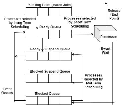
Fig.1. Scheduler activity simulation diagram

Basically, there are some criteria for scheduling of processes mentioned [15] such as increasing the number of throughput and enhancing maximum CPU utilization, decreasing turn-around-time, reducing waiting-time and minimizing context-switching. Round robin is the algorithm that is really efficient for scheduling of processes in preemptive manner [16]. In order to enrich these criteria a proficient RR algorithm is essential because it keeps the performance of preemption realistic and sustained. To enhance the efficiency in the field of CPU scheduling, a new round robin algorithm has been introduced in this paper based on the maximum difference of two adjacent consecutive processes present into the ready queue [17].

Enormous number of round robin algorithms is presented with different types of time quantum that can be determined dynamically or statically. The performance of RR algorithms depends on the determination of an outstanding time quantum. In this paper a proficient round robin algorithm has been proposed where the time quantum has been determined dynamically based on the maximum difference among the differences of adjacent consecutive process burst times. The presented algorithm is comparatively better and efficient as compared to other mentioned RR algorithms in this paper. The proposed algorithm has fulfilled the mentioned criteria mentioned in above. The rest of the paper is decorated by Related Work in section II, Proposed Algorithm in section III, Experimental Setup and Result Analysis is demonstrated in the section IV and section V shows and describes the conclusion.

• II.    Related Work

Multitasking as well as Multiprocessing is one of the most noticeable phenomena in terms of computer resource allocation [1]. To manipulate in this regard, this operations a perfect scheduling is required by which the reliability and efficiency as well as allocation of resources will be implemented. The effective scheduling of process as well as the allocation of resources is one of the desired concepts in this modern computing technology in the field of cloud computing and CPU. To enhance the performance, the Time Quantum must be optimum [2].

Managing the precise allocation of resources is highly required subject in this modern era. It enhances the accessibility of resource whenever one wants or wherever one wants. The Round Robin efficient algorithm for resource distribution is extensively utilized in terms of increasing the proficiency and effectiveness, accessibility, portability of resources [3].

There are some strategies to develop and introduce a scheduling algorithm. Various numbers of scheduling algorithms had been developed by means of following these strategies for process execution [4]. Among these some algorithms allow preemption and some other allows non-preemption. The common strategies are First Come First Serve, Shortest Job First, Priority Based Scheduling Algorithm and Round Robin. Sometimes a scheduling algorithm can be developed by merging two or more strategies among these [5].

To enhance the performance of the CPU scheduling, there are variety number of algorithms are developed. FCFS is commonly used scheduling algorithm which was preliminary utilized for scheduling [6]. This algorithm is good in general sense but it sometimes provides importance the jobs which are unimportant that means a process that is required to execute further can be executed first than other required processes [7]. Shortest job first (SJF) is another popular scheduling algorithm but creates starvation problem in process scheduling. The main difficulty of this algorithm is to determining the next of the next CPU burst time [8].

With a view to maintaining preemption approach priority based scheduling strategy has been welcomed in which processes are prioritized according to their requirement [9]. The both scheduling algorithm SJF and priority based scheduling also causes starvation in terms of low priority based processes [10]. Prioritization is an activity to prioritize the processes according to the demand during execution. Starvation can be caused here [11]. Round Robin scheduling algorithm is the best algorithm for process scheduling because it allows preemption. In round robin, time quantum is the most considerable term [12]. The time quantum can be determined in various ways such as considering median value, partial average etc. Even the time quantum can be fixed after first or second iteration [6, 13].

The strategy of scheduling is the best subject in terms of creating better effectiveness on the increment of efficiency in the allocation of resources like CPU [13]. Quantum size is required term in Round Robin algorithm that is enormously utilized in scheduling here context switching number, amount of waiting time in average and turn-around time in average are inextricably involved. The involvement of these terms can be the issue of decrement of the performance or the increment of performance [14]. Multitasking as well as multiprogramming are the key concepts in our modern technology. Scheduling algorithms are generally used with a view to managing these tasks. To schedule each process a quantum time related with turn-around-time besides burst-time as well as the quantum time is approximately optimal. Improved Round Robin algorithm is commonly used to do such scheduling proficiently and precisely [15].

Sometimes the SJF and RR both algorithms are combined together to determine a time quantum and build up an excellent scheduling algorithm [16]. Ajit singh et al. introduced a round robin algorithm where the time quantum becomes twice than its previous time quantum [17]. Mean average value has been evaluated for determining a dynamic time quantum [18]. Modulus technic has been also been used to define a time quantum for round robin [19]. Mohanty along with other researchers also developed various round robin algorithms for process scheduling to increase the performance [20]. Priority based algorithm and RR have been accumulated together to build up an algorithm and another is the combination of SJF and RR [21].

Related work section demonstrates enormous number of utilizations of round robin in various purposes. Round robin is widely applied due to its preemption feature that means it allows all processes during execution for a certain period of time according to time quantum. In this paper we have also endeavored to determine proficient time quantum to improve the performance of round robin for scheduling algorithm.

• III.    Proposed Algorithm

The proposed algorithm focuses on the determining the time quantum which increases the performance of round robin scheduling algorithm. Our proposed algorithm has been devised on the basis of median value of processes [18] and considering the maximum difference among differences of adjacent consecutive processes into the ready queue. In this approach, the burst time of all the processes are sorted in ascending order in the ready queue. Then the time quantum is calculated using the equations below.

diffuA = р,+:+р,(1)

MAX_DIFF = MAX(DIFF[i])(2)

TQ = MBT + MAX_DIFF(3)

Here, TQ = Time Quantum, MBT = Middle Burst Time and MAX_DIFF = Maximum Difference among the Differences of two consecutive processes. The proposed methodology has a couple of advancing feature and considerable aspect. The first advancing feature is that it calculates differences among consecutive processes into the ready queue after sorting. By this strategy, it is possible to measure how much time is more required to be executed among processes into the ready queue. This technique discovers a way to calculate the range of the execution and burst times of all processes into the ready queue that is highly advantageous in term of determining an optimal and efficient time quantum for the execution of these processes. Second advancing strategy is calculating maximum difference among these differences because it is the maximum distance of the range that covers all other more required burst times which is also beneficial for setting up a proficient time quantum. Calculating differences of burst times and maximum difference among these are the aspects that specify the betterment of the proposed algorithm than others.

In order to make the proposed algorithm more explicit, the steps of the proposed algorithm described in the following.

• >    Step - 1: According to burst time, all the processes had been sorted in ascending order.

• >    Step - 2: All the differences of two adjacent consecutive processes had been calculated.

• >    Step - 3: The maximum difference among these differences had been calculated.

• >    Step - 4: The median value among sorted

processes had been calculated.

• >    Step - 5: After that the time quantum had been calculated which is the summation of maximum difference and median burst time.

• >    Step - 6: if (process burst time - time quantum) = 0, the process will be terminated.

• >    Step - 7: if (process burst time - time quantum) != 0, the process will be shifted at the tail of the ready queue and step 6 and 7 will be continued until the process completes its execution.

• >    Step - 8: Average Turn-Around-Time and average Waiting-Time had been calculated.

The available processes into the ready queue will be considered during calculating or determining the time quantum. Since the processes will be sorted after their arrival according to their arrival time, the second process will be higher than first process. For this reason, the differences will be calculated successively Pi from Pi+1. After that the maximum difference among these differences will be identified. The Fig. 2 represents the pictorial representation of the consecutive steps of the execution of processes by CPU according to time quantum. In the figure, it has been demonstrated that all processes require to be sorted in ascending order. The time quantum of the proposed algorithm has been determined dynamically based on the maximum difference among the differences of two adjacent consecutive process burst times.

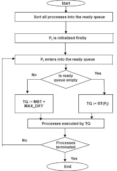
Fig.2. Consecutive Steps of Process Execution

The mechanism of execution of the proposed algorithm has been evaluated. To analysis we arrange 4 processes P1, P2, P3, P4 having distinct burst times such as 34, 19, 21, 46ms respectively. All processes have arrived at zero millisecond. Firstly, the processes have been arranged in the ascending order P2, P3, P1, P4. Then the differences have been calculated 2, 13, 12 respectively. The maximum difference has been calculated 13. After that the middle burst time has been calculated based on the equation [2]. Here MBT = (21 + 34)/2 = 27 . The time quantum will be MBT (27) + MAX_DIFF (13) = 40 . The Table 1 represents the execution simulation over the data set with Gantt-Chart.

Table 1.Simulation of execution through Gantt-Chart

P2	P3	P1	P4	P4
19	40	74	114	120

>      40   ◄---------- -> 6

When the execution starts, the P2, P3, P1 will be completed and eradicated from the ready queue. After the first execution, the second TQ = 6. Eventually, P4 enters into the ready queue and completes its execution. According to the proposed algorithm, the completion times of processes are 19, 40, 74, 120 and waiting times are 0, 19, 40, 74. The average turn-around-time is 63.25, average-waiting-time is 33.25 and context switching is 5.

The appropriateness of the proposed algorithm has also been measured for the processes at which all burst times are equal for them. To evaluate the performance we decide 5 processes all having equal burst time such as P2(32), P4(32), P1(32), P5(32) and P3(32). After entering all processes into the ready queue, the sorting will be occurred. After sorting in ascending order, first process will be executed because their burst times are equal. Here, differences between two consecutive processes are zero and the maximum difference is 0. After sorting, all processes have been arranged in P1, P2, P3, P4, P5 order. In this case, the middle burst time is 32. So, MBT=32 based on equation [2]. Finally time quantum will be MBT(32) + MAX_DIFF(0) = 32 which is equal to the burst time of all processes reached into the ready queue. It can be stated that the time quantum is equal to the burst time based on the proposed methodology when burst times of all processes are equal. For the mentioned dataset, average turn-around time is 96, average waitingtime is 64 and the number of context switching is 5.

Algorithm 1: Determination of Time Quantum (TQ)

• 1.    Input: ВТ (Burst Time), N (Number of Processes)

• 2.    Output: TQ (Time Quantum)

• 3.    Begin if N is Odd do

• 4.    Midpoint *- (N + l)/2 //Midpoint: Index of the middle value

• 5.      МВТ*- ar r(Midpoint).ВТ

• 6.    Fori=ltoNdo

• 7.    MAX_DIFF <- Find the max difference among ВТ

• 8.     End For

• 9.     TQ <- МВТ + MAX_D1FF

• 10.    Eke If N is even do

• 11.    Midpoint«- N/2

• 12.    МВТ <- (ar r(Midpoint) .ВТ + arr(Midpoint + 1) .ВТ)/2

• 13.    Fori=ltoNdo

• 14.    MAX_DIFF <- Find the max difference among ВТ

• 15.   End For

• 16.    TQ <- МВТ + MAX_D1FF

• 17.    End If

The most considerable term of the proposed RR algorithm is a proficient time quantum. When the first process arrives, the time quantum becomes equal to the first burst time. After that the time quantum is changed shown in Fig. 2. The proposed methodology for determining TQ is comparatively outstanding because TQ is determined dynamically based on the maximum difference. When a new process comes into ready queue, the differences of two adjacent consecutive processes are calculated and the maximum difference is determined among these. Finally, TQ is calculated by means of addition between Middle Burst Time and Maximum Difference determined in Algorithm-1.

Time quantum is an extraordinary portion of time can be called time slice. CPU schedulers capture processes to execute appropriately according to the defined time quantum in multitasking system [16]. Time quantum can be two types one is fixed time quantum and another is dynamic time quantum. Time quantum is inextricably related to preemptive CPU scheduling. An efficient time quantum enhances the performance of CPU scheduling algorithms [17]. There are eye-catching variations in round robin algorithm based on the time quantum. Time quantum sometimes is determined dynamically and sometimes the time quantum is fixed.

The Algorithm-1 is the demonstration of the contribution of the proposed methodology. We have tried to determine a time quantum that is restively efficient and will be determined dynamically. The line 10 and 27 express the midpoint determined according to the number of processes. In the line 11 and 28 holds the middle burst time. Form line 12-15 and 29-32 finds the differences among all available processes into the ready queue. Then the maximum difference among these differences has been calculated in the line 16-23 and 33-40.

Finally, the special and outstanding time quantum has been calculated that controls the execution of processes by the addition of middle burst time and maximum difference among the differences of two consecutive adjacent processes.

• IV.    Experimental Setup and Result Analysis

The proposed algorithm had been developed and illustrated with a view to increasing the performance of scheduling in the field of maximum throughput, maximum CPU utilization, reducing turn-around-time (TAT), minimizing waiting-time (WAT) and contextswitching (CS). Basically, there are two types of processes such as having equal arrival time (0) or different arrival times. The proposed algorithm had been implemented with C++ along with 64bit windows10 operating system, with Intel core i7, 4GB RAM. In this experiment two data set having same arrival time and different arrival time had been used. Result has been enrolled through table and demonstrated through graph. Process execution has been shown through Gantt-Chart.

Table 2.Processes with zero arrival time (case study – 1)

Processes	Arrival Time	Burst Time
P1	0	105
P2	0	60
P3	0	120
P4	0	48
P5	0	75

Table 2. represents a data set having 5 processes P1, P2, P3, P4 and P5 having distinct burst time 105, 60, 120, 48 and 75 with zero arrival time. According to the proposed algorithm, firstly all the processes will be sorted in ascending order. After sorting the processes will be arranged in the ready queue in an order like P4 << P2 << P5 << P1 and P3 and all these processes are ready to be executed.

Now the differences of the two adjacent consecutive processes are DIFFS = {12, 15, 30, and 15}. The maximum difference among these differences is 30. So MAX_DIFF = 30. The number processes is 5. The midpoint is 3. The median value among these burst time is 75. Finally, the time quantum is 75 + 30 = 105. After first execution P4, P2, P5, P1 complete its execution but P3 does not complete its execution. So P3 will move at the end of the tail of the ready queue with its remaining time. The next time quantum is 15 according to the remaining time of the processes. Eventually, P3 completes its execution and is removed from the ready queue.

Table 3.Simulation through Gantt-Chart of case study -1

P4	P2	P5	P1	P3	P3
48	108	183	288	393	408

> TQ = 105 ч             15

Based on the proposed algorithm, the sequence of processes according to completion of execution is P4 >> P2 >> P5 >> P1 >> P3. The completion time of these processes are 48, 108, 183, 288, 408. The average turnaround-time is 207 and average waiting-time is 114.4. According to the Gantt-Chart at Table 3, the number of context-switching is 6.

Table 4.Processes with different arrival time (case study – 2)

Processes	Arrival Time	Burst Time
P1	0	45
P2	5	90
P3	8	70
P4	15	38
P5	20	55

Table 4 also represents another data set also having 5 processes P1, P2, P3, P4, P5 having distinct burst time 45, 90, 70, 38 and 55 and different arrival time. Here, P1 process arrives first in the ready queue and the time quantum is 45. After that P1 completes its execution. On that moment, all processes arrive into the ready queue. According to the proposed algorithm, the processes will be sorted in a sequence like that P4 << P5 << P3 << P2 and they are ready to be executed. Now the differences of the two adjacent consecutive processes are DIFFS = {17, 15 and 20}.

The maximum difference among these differences is 20. So MAX_DIFF = 20. The number of processes is 4. The midpoint is 2th and 3rd processes. The median value among these burst time is (55 + 70)/2 = 62. So the MBT = 62. Here, the second time quantum is (62 + 20) = 82. After this execution P4, P5, P3 complete its execution but P2 does not complete its execution. So P2 will move at the end of the tail of the ready queue with its remaining time. The next time quantum is 8 according to the remaining time of the processes and P2 completes its execution and is removed from the ready queue.

Table 5.Simulation through Gantt-Chart of case study - 2

P1	P4	P5	P3	P2	P2
45	83	138	208	300	308

45  -----------------►    82 N            8

Based on the proposed algorithm, the sequence of processes according to completion of execution is P1 >> P4 >> P5 >> P3 >> P2. The completion time of these processes are 45, 68, 118, 200, 303. The average turnaround-time is 146.8 and average waiting-time is 87.2. According to the Gantt-Chart at Table 5, the number of context-switching is 6.

To evaluate the performance of the proposed algorithm, an experiment was conducted with two different data sets having zero arrival time and distinct arrival time by comparing some other existing proposed round robin algorithm. The datasets were selected from existing literature [16] to avoid biasness of the experiment. Each dataset contains 5 processes with different burst times.

The proposed algorithm is comparatively excellent even if the number of processes is increased. Here 25 as time quantum is determined to analysis general RR. Only these processes are considered which are CPU bound. 5

distinct processes have been considered for every case. Arrival Time (AT) and Burst Time (BT) are known before execution. Ajit Singh et al. [10] have introduced a RR algorithm in which the TQ becomes double. We have considered it R.R-10 because it has been referred at 10th place in the reference section.

Table 6. Processes with zero arrival time (Data set-1)

Processes	Arrival Time	Burst Time
P1	0	105
P2	0	85
P3	0	55
P4	0	43
P5	0	35

There is a comparison table over the above Table 6 mentioned dataset-1. The comparison occurs on the proposed algorithm against general round robin (RR), DQRRR [9], IRRVQ [4], SARR [18], R.R – 10 [10], MRR [6], DABRR [16]. The comparative terms are Context-Switching (CS) represented in the third row, average Waiting-Time (WAT) presented in forth row and average Turn-Around-Time (TAT) demonstrated in fifth row in the Table 7.

Table 7. Comparison on proposed algorithm (PRR) against RR, DQRRR, IRRVQ, SARR, R.R-10, MRR, DABRR for dataset-1

Alg	RR	DQRRR	IRRVQ	SARR	R.R - 10	MRR	DABRR	PRR
TQ	25	55, 40, 10	35, 8, 12, 30, 20	50, 40, 10	25, 50, 100	70, 25, 25	64, 31, 10	85, 20
CS	16	8	15	8	12	8	8	6
WAT	209.4	144.8	142	185.8	224.8	106.8	105.6	92.8
TAT	274	209.4	206.6	250.4	289.4	171.4	170.2	157.4

Table 8.Processes with different arrival time (Data set-2)

Processes	Arrival Time	Burst Time
P1	0	95
P2	2	75
P3	4	60
P4	8	43
P5	16	26

There is another comparison table over the above Table 8 mentioned dataset 2. The comparison occurs on the proposed algorithm against general round robin (RR), DQRRR [9], IRRVQ [4], SARR [18], R.R – 10 [10], MRR [6], DABRR [16]. The comparative terms are Context-Switching (CS) represented in the third row, average Waiting-Time (WAT) presented in forth row and average Turn-Around-Time (TAT) demonstrated in fifth row in the Table 9.

Table 9.Comparison on proposed algorithm (PRR) against RR, DQRRR, IRRVQ, SARR, R.R-10, MRR, DABRR for dataset-2

Alg	RR	DQRRR	IRRVQ	SARR	R.R – 10	MRR	DABRR	PRR
TQ	25	95, 51, 16, 8	95, 26, 17, 17, 15	95, 51, 16, 8	25, 50, 100	95, 49 25, 25	95, 51, 16, 8	95, 68, 7
CS	14	8	11	8	9	8	8	6
WAT	191	138.4	133.8	172.4	197	124.6	125	114.8
TAT	250.8	198.2	193.8	232.2	256.8	184.4	184.8	174.6

Our proposed algorithm is experimentally better shown in comparison Table 7 and Table 9. If the number of data set is increased with large number of processes, the proposed algorithm will also provide outstanding result. Result and discussion section is the mirror of the proposed methodology. In this section, comparative consequences had been reveled on the fair of proposed algorithm against other Round Robin Algorithms. Proposed Algorithm that means proposed method had been applied over various data sets with a view to testing its efficiency than other algorithms. Undoubtedly excellent and desired performance had been performed by the Algorithm. By the Fig. 3 and Fig. 4 two consecutive graphical representations express the proficiency of the proposed methodology in terms of average waiting-time and average turn-around time over dataset-1 and 2.

In a concise statement, it is possible to say that the proposed algorithm is comparatively excellent and preferable in terms of decreasing turn-around time, waiting time and context-switching than other. Eventually, it is decided that the proposed algorithm is fully optimized and essential in enhancing the performance of a system regarding scheduling of CPU in the operating system. After getting inadequate experience from the proposed algorithm and result analysis it is our proposed methodology is eligible for CPU scheduling with a good conduct.

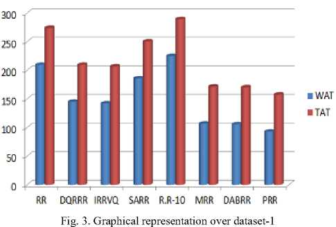
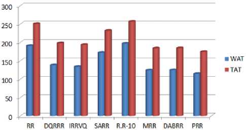
Fig. 4. Graphical representation over dataset-2

• V.    Conclusion

CPU scheduling is a great challenge indeed to enrich and make the best and significant utilization of CPU in the operating system. The proposed algorithm and methodology is nothing but a trivial effort with a view to increasing the system performance as well as the effective use of resources. After a close attention, it is completely explicit that our proposed optimized Round Robin Algorithm Based on maximum difference between two adjacent consecutive processes is comparatively appropriate, eligible as well as better than other Round Robin Algorithms. This proposed method is concerned not only performance but also minimizing the turnaround-time, decreasing the waiting-time, increasing the number of throughput and so on. By applying and deploying our program it is possible to enhance and improve the process allocation through system appropriately. Since optimal time quantum is the most important term pertaining the increment of the proficiency in the performance of a system. The system's performance will be more efficient by determining an optimal time quantum. Our future objective is to determine an optimal time quantum with a view to enhancing the system's performance. The proposed algorithm and methodology has a limitation in terms of prioritization without causing starvation when burst times of all processes are equal. A program is a collection of processes. If burst times of all processes into the ready queue of the program are equal, first process has been executed first based on the proposed algorithm. It cannot be fair at all times. It is standard to prioritize the proposed based on the demand and requirement. Though priority scheduling algorithm had been announced in this case but it causes starvation where burst times are not equal or equal. So, it should be determined which process is highly demanded among these during execution of program and should build a demand sequence of the processes for the program. Our future work is to determine the demanded sequence of processes of the program during execution when burst times are equal into the ready queue. It will also enhance the performance of the proposed algorithm.