Development of Algorithm to Reduce Shadow on Digital Image

Published Online November 2016 in MECS

In object extraction, presence of shadow contributes to falsification of the object’s shape, inaccurately measured of geometrical properties and also creation of false adjacency between different objects on images [1]. The wrong classification of the shadow as foreground can occur easily since the intensity values of the shadow region are typically differ significantly from the background values. The existence of the shadow can cause objects merging and shape distortion that may result in the failure in object detection procedures or object misclassification [2].

It is possible that the shadow been classified as a part of the foreground objects itself. As a consequence, both objects and the shadow are detected at the same time and therefore being merged together into a single blob. Due to this reason, there is a higher possibility of object undersegmentation to occur. This is because different objects tend to get connected via shadow, which causing both object and shadow got merged together. This greatly affects geometrical properties and appearance of the object to be detected [3]. Shadow can cause inaccuracy in some applications, such as the applications for plant leaves segmentation [4], license plate recognition [5], gait recognition [6,7], analysis of remote-sensing images [8,9], classification of objects from video surveillance system [10], underwater object detection [11] and clustering [12].

Shadow removal presents us a whole different challenge as shadow detection. The target shadow region cannot be simply removed, but has to be effectively replaced with data sampled from the remainder of the image itself. This is done to present new color values of the replaced shadow region that looks reasonable to human eyes. However, the approach to replace shadow region by replicating the texture would require an exhaustive search of appropriate texture patches throughout the image and hence brings up computation load and processing time [13]. This problem worsened upon detection of large-sized shadow region. Filling of large target shadow region is harder due to higher possibility of occurrence of spatial interaction of multiple textures within the region, ending up with mutual influences between several textures. Some restoration algorithms which fill up shadow region via diffusion, could introduces blur that is more observable when it comes to filling of the large target region. These problems, hence limit the capabilities of some algorithms to process shadow region of small size only [14].

Salient features that can be extracted from digital image such as contrasts, sharpness and structure of the color are essential to carry out shadow detection and removal. This project mainly utilizes image information, especially intensity information, with the assumption that the shadow areas are being less illuminated than the surrounding areas [15]. Unfortunately, such information may not be found in a grayscale image. Therefore preprocessing such as RGB approximation and the addition of chrominance and luminance would be needed [16]. Thus, for this project, digital color image would be used as input instead of grayscale image, allowing more effort to be put on development of shadow detection and removal algorithm. As shadow detection and removal covers a wide scope of research, this project aims to address problems of shadow detection and removal given an input of a single still image. This project will use single digital color image as input. The developed algorithms will work without the need of referral image. Furthermore, the development of shadow reduction algorithm does not cover for application on video sequences. Therefore, temporal information will not be considered in this research. Deep learning method for shadow detection and removal, such as the one used by Khan et. al [17], will not be employed in this research.

The remainder of the paper is outlined as follows. In Section II, literature review on shadow modelling and CIE Lab color space are presented. The two proposed algorithms are described in Section III. Then, the results from all proposed algorithms are presented and compared in Section IV. Lastly, the Section V concludes the paper.

^ t ^{( x} , y )

[ C_P cos ф + C A t C A

: No shadow

: Umbra

• II.    Literature Review

This section presents some fundamental theories related to this research. This section is divided into three subsections. The first subsection presents the shadow modelling. Then, the next subsection shows the color space conversion. The last subsection gives some review of some basic morphological operations.

• A.    Shadow Modelling

An image can be segmented into object, object castshadow and background. Two main branches of shadow region are ‘self’ shadow and ‘cast’ shadow. Self shadow is shadow region generated on an object when the object itself is obstructing light from the light source. On the other side while the same object is blocking the light, cast shadow region will occur on, instead of the object itself, but on other objects in the same scene. For cast shadow, it can be further sub-divided into umbra and penumbra region. Umbra is formed when the light source is completely blocked, whilst penumbra is formed when the source is partially blocked [18].

To briefly explain the basis of shadow detection algorithm, reflection model is used to describe the luminance ( i.e. the brightness) of a point, at the two dimensional image position ( x , y ) and time instant t . Reflection model as given by (1) describes luminance, W t ( x , y ) [18]:

W t ⁽ x, У ) = ^ t ⁽ x , У ) P t ⁽ x , У )              (1)

where ф is angle enclosed by light source direction and surface normal.

• B.    Color Space Conversion

It is a fact that the human retina consists of three types color photo receptor cone cells. Each type of this cone cells has difference spectral sensitivities. As a result, human color vision is trichromatic, or in other words, a color that experienced by our eyes can be characterized by three real numbers. Another photo receptor cells named rod are present too. However, statistics related to them are ignored as they do not contribute to perception of color [20].

In general, color space is notation by which color can be specified by points in three-dimensional arrangements of color sensations. Based on the work done by Tkaleie and Tasie [21], it is proposed that color space can be grouped into three main categories. These categories are (1) HVS based color spaces, (2) Application specific color spaces and (3) CIE color spaces.

International Commission on Illumination (abbreviated as CIE) has created CIE XYZ color space in year 1931 by standardizing XYZ values as tri-stimulus values to describe levels of perceptible visual stimulus. It is regarded as device independent and functions as a standard reference [11]. With all three stimulus X, Y and Z defined, it is possible to derive CIE xy chromatic coordinates from it with (4) and (5), as the two chromatic coordinates x and y are used to specify “pure” color under the absence of illumination [20].

where p ( x , y ) is reflectance component of the object surface and ^ ( x , y ) is illumination component from light source. The illumination component, ^ ( x , y ) is the amount of light power per receiving object surface area, which can be defined by (2).

X

Y

C_PN_X L_x „ + C_A

P x , y x , y     A

^ t ( x , y ) = U , y C p N x , y L

' x , y ⁺ C A

C A

: No shadow

: Penumbra

: Umbra

where L is direction of light source with object surface normal, N is object surface, C is intensity of direct light, C_A is intensity of ambient light and Л_х is transition inside the penumbra (0 <  X _{x y} <  1) . There are also methods that use a simplified version of illumination and shadow model, for example in work done by [19], which ignore shadow penumbra. The simplified formula used in mentioned work define EA ( x , y ) by using (3):

CIE Luv is color space which main goal is to create a perceptually uniform color space, in which two main constraints (chromatic adaptation and non-linear visual response) are to be taken into consideration [21]. L components gives illuminance while u and v components provide information on chromaticity values of image. Prominence of red components and prominence of green components over blue are indicated by negative values of u and v components respectively. Equation (6), (7) and (8) show conversion of Luv from XYZ color space [22]:

Гу) 3

V Пп )

- 16

where

v = 13 L ( v - v n )

'

u

4 X

X + 15 Y + 3 Z

U n =

4 X n

X n + 15 Y n + 3 Z n

■

v

9 Y

X + 15 Y + 3 Z

v n =

9У

n

X_n + 15 Y n + 3 Z_n

CIE Lab color space consists of three channels, which are L Channel, a Channel and b Channel. L Channel provides lightness information, ranging from 0 to 100 which portrays distinct shades from black to white. Derivation of Lab color space is performed by transforming XYZ using (13) and (14). For Lab color space, L component is defined using (6), the same equation which defines L components for Luv color space too. Tristimulus values X_n , Y_n and Z_n are those of the nominally white object-color stimulus [15].

a = 500

^f X ) 3 I X n )

b = 200

Y

Y n

In general, a Channel represents red to green ratio while b Channel represents yellow to blue ratio. Both a Channel and b Channel ranging from -128 to +127 (256 levels). Euclidian distance between two colors in this color space is strongly correlated with human visual perception, which enables it to describe all the colors visible to human eyes. CIE Lab color space normalizes its values by the division with the white point [23].

• C.    Morphological Operations

Mathematical morphology is the name of a collection of operators based on set theory and defined on an abstract structure known as infinite lattice. Examples of morphological operators are erosion, dilation, opening, closing, rank filters, top hat transforms and more. Main application field for the tool of morphological transformation would be image analysis and image enhancement. Morphological transform would be defined as mathematical structure that can formalize an ordering relation, and the two basic operations infimum (л) and supremum (v). Infimum is the greatest lower bound while supremum is the smaller upper bound. The most basic morphological operation are dilation and erosion. Erosion, En and dilation, dN of the f (p) can be defined by (15) and (16), respectively [24].

E Nf(P) = |^ f(P IP e NG(P) ■ f(P)}

^Nf(P) = {v f (P | P e NG(P) и f (P)} where NG (p) is set of neighbor pixel p with respect to grid G. Opening operator ( Yn ) is result of erosion followed by dilution, as given by:

YNf (P) = SNENf (P)

Discontinuous regions can be filled by using dilation operation but increase the detecting region, while erosion can restore the region size. On the other hand, closing operator ( ф N ) is done by carry out dilation first then followed by erosion:

P _N ^{f (} P ) = e N S Nf ⁽ P )            (18)

Erosion can be used to eliminate noises but the detection region will become smaller, while dilation can help to restore. Opening operator cuts peak while closing operator fills up small valleys. Residual between filtered image and original image is observed in top hat (given by (19)) or inverse top hat transform (given by (20)) [25].

Г f ( P ) = f ( P ) - Y Nf ( P ) = f ( P ) - S n E nJ ( p )   (19)

^Г — 1 ^{f (} P ) = ^{f (} P ) ^- ^ N^{f (} P ) = ^{f (} P ) ^{- E} N ⁵ N^{f (} P ) ⁽²⁰⁾

Opening and closing operators are used to smoothen ragged edges and close up small holes in the regions.

• III.    Proposed Algorithms

The proposed shadow removal algorithm consists of three major processes being carried out in sequence. These main processes are shadow detection, shadow reduction followed next by shadow edge correction, as shown in Fig. 1. An RGB image will be acquired as input and converted into its equivalent in Lab color space before any processing is carried. Through analysis on the input Lab image, shadow regions are detected and shown in binary shadow mask, S as white region.

With shadow region being identified, shadow reduction is then carried out by replacing shadow pixels with color values that seems reasonable to human vision. Technique used for shadow removal is multiplying the shadow region by appropriate constants which eliminates illumination reduction that result in presence of shadow. This is done with input of Lab image, binary shadow mask and also tuning input (i.e., VL, Va and Vb).

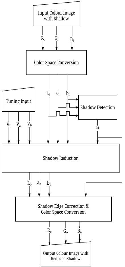
Fig.1. Block diagram of the project.

This stage will result in output Lab image. Lastly shadow edge correction is performed on output Lab image before converted back as RGB color image. In this project, shadow region needs to be identified first while minimizing occurrence of a situation where objects are being misclassified as shadow region. To avoid such situation, accuracy of shadow detection algorithm should be emphasized which assures better result when it comes to shadow reduction. Shadow removal needs to be performed without deterioration of texture consistency of the image. Two methods are proposed for this project, which are marked as Algorithm A and Algorithm B for identification purpose.

• A.    Algorithm A

This section presents an approach to detect shadow region which is adapted from [15] and some modifications are applied before it is implemented for this project. First, RGB image is converted to Lab color space before going through any further processing. When an RGB color image is converted to its equivalent image in Lab color space, color information which consists of red, green and blue components are now accessible through two color channels of Lab color channels, which are a -plane (red-to-green ratio) and b -plane (yellow-to-blue ratio). For shadow identification, not only lightness information but also color information is used for analysis. After converting color space of the image, mean values in a -channel and b -channel ( a ^~ and b ) are computed based on converted image. The summation of both mean values are used to determine which subroutine works better. This is done by comparing the sum with a threshold value.

With reference to [15], for an image of M x N pixels, pixels which its L -channel value is less than difference of the previously calculated mean value in L -channel and one-third of standard deviation in L -channel can be classified as shadow pixel. This is shown in (21) for better understanding.

S ( x , y ) = f

^: L ( x , y ) < ~ - ^ L

.

: Others where ct^ is standard deviation in L-channel:

1     M x N.    ~2

^L = (M x N)-1 П=1 Ln - LI

~ and L

is mean of L -channel values of all image pixels

~

L =

1   M x N

I L_n

If summation of both mean values in a -channel and b -channel is equal or less than the specified threshold, a shadow mask with symbol S will be generated using (21) where shadow pixels are shown as white region.

For the case where summation a ^~ and b ^~ exceeds the specified threshold, (24) is used instead of (21) for the purpose of shadow pixel classification. To classify a pixel as shadow pixel, both L -value and b -value of the pixel have to be less than L ^~ and b ^~ previously computed, as shown in (24):

S ( x , y ) =

: L ( x , y ) <  L , n b ( x , y ) <  b

: Others

This algorithm will be used to examine every pixel and classify them as either shadow pixel or non-shadow pixel.

This is carried out row-by-row until the last pixel of the image is examined. Once this procedure has completed, a binary shadow mask will be obtained and will be used for further processing.

The algorithm now proceeds to shadow reduction with shadow mask S previously generated based on the work done by [26], upon completion of shadow detection. Sampling of illumination changes between shadow region and non-shadow region is done by sampling a nonshadow pixel and shadow pixel both located at opposite side of the shadow boundary, in horizontal direction for this project.

Let P be array of last pixels right outside the shadow region and S be array of first pixels right inside the shadow region [26]. Constant C used for shadow attenuation can be calculated by using (25):

с ( k ) =

. N J Pi ⁽ k ) - Si ⁽ k ^)] i =0 __________________

N

where k is number of channel for Lab color space, N is total number of shadow boundary pixels. Appropriate constants has been determined by calculating mean of difference in P vector and S vector for all three channels. Shadow region is then reduced by adding the constants obtained to it in order to minimize the difference across the shadow edge.

After shadow removal is carried out, occurrence of error around shadow boundary is likely to happen and therefore needs to be overcome. As shadow detection occasionally misses out small portion of shadow region around shadow edge, uneven illumination such as dark circular shadow around the shadow edge would still occur even after shadow removal is done. Two interpolation methods that have been tried out in this project are scattered data interpolation and onedimensional data interpolation. Through experimental approach, one-dimensional data interpolation is proven more suitable to be used for this purpose.

• B.    Algorithm B

Algorithm B is proposed with adaptation from work done by [27] with modifications being made before implementing it for this project. For Algorithm B, segmentation of potential shadow region is carried out by thresholding on L channel. For this project, the threshold for L channel ( T ) is set to be at 55 out of the range of 0 to 100.

With aid of color thresholder apps in Matlab, it is observed that thresholding of a channel at Ta =-10 is effective for shadow region with green-colored background. On the other hand, thresholding of b channel at Tb = 10 works better for shadow region with yellowcolor background. Based on observation on input image, one has to choose of applying thresholding at Ta = -10, Tb = 10 or no thresholding in some case. Thresholding of a channel and b channel for shadow detection are according to (26) and (27) as shown below:

1,

S ( i , j ) = 1 ’

1 0,

1,

S ( i , j ) = 1 n

1 0,

: L ( i , j ) <  Tl &  a ( i , j ) <  T_a : else

^: L ⁽ i , j ) <  ^T _L &  ^{b (} i , j ) <  ^Tb : else

For case where shadow region located in both yellow and green colored background, none of thresholding of a channel and b channel are applied to ensure shadow region of both yellow and green colored background are detectable. This step is carried out based on (28):

S«,j) = ( 1 : L(“) <  TL (28) ^ 0, : else

Similar to Algorithm A, morphological open and close operations are done on final shadow to eliminate noises followed by area-based thresholding. Although different shadow detection method are implemented in Algorithm A and B respectively, both of them perform similar algorithm to reduce shadow region. This is then followed by shadow edge correction using one-dimensional data interpolation.

• IV.    Experimental Results and Discussions

(b)

(a)

This section is divided into three subsections. The first subsection gives the preliminary experiment results for Algorithm A. Then, the next subsection presents the preliminary experiment results for Algorithm B. The last subsection presents the comparison of the results.

• A .    Preliminary Experiments on Algorithm A

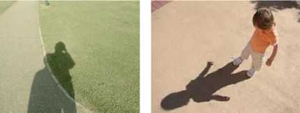
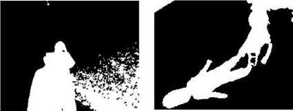
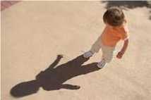
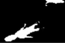
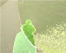
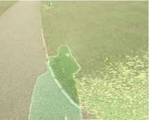
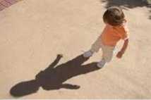
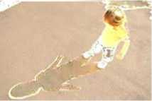
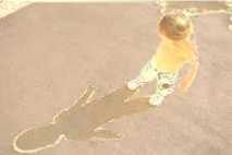
In Fig. 2(a), it is observed that there are many small shadow spots that a slightly less illuminated at the bottom-right portion of “Field.jpg”. Therefore, in Fig. 3(a), shadow regions are detected almost correctly with noises introduced at bottom-right portion of this image. In Fig. 3(b), the shadow detection result for “Girl.jpg” shows misclassification of object as shadow region due to its lower illumination compared to its surrounding region. However, the shadow regions are still detectable using this method.

(a)                                     (b)

In this subsection, tuning of constants for Algorithm A is carried out to optimize the performance of shadow removal (i.e., the stage after shadow detection). Three constant, each representing each channel of Lab color space, will be varied and the suitable one will be selected based on the results. Lets values added to constant for L channel, a channel, and b channel be V_L,A , V_a,A , and V_b,A respectively.

First, the value of V_L,A is varied for six values (+10, +20, +30, +40, +50 and +60). Tuning for L channel is carried out first by increasing values of V L,A by 10, from 0 to +60. It is observed that the illumination of shadow region increases as values of V L,A become higher. However, texture information of shadow region starts to lose when V_L,A goes beyond +30, hence V_L,A equal to +30 is chosen.

Next, tuning of the a channel is carried out. Similar to L channel tuning, the valuie of V a,A is varied for six values. Since range of the channel is from -128 to 127, V a,A is varied by increasing it by five, starting from -15 to +15, except zero (-15, -10, -5, +5, +10, and +15). It was observed that the color of replaced shadow region shifted towards red color when V_a,A is increased by five from 0 to +15. On the other hand, replaced shadow region has become less in red color when V_a,A less than zero. From our observation, V a,A =-15 gives the best results, and thus we choose V a,A equal to -15.

Then, tuning of b channel is carried out. Similar to tuning of a channel, V b,A is varied by increasing it by five starting from -15 to +15. It is observed that replaced shadow region becomes darker and shifted towards blue color as V_b,A is reduced to less than zero. When V_b,A is increased from 0 to +15, replaced shadow region is now shifted towards orange colour, but such changes are not significant. Since changes in V b,A is not significant, V b,A equal to zero is selected, which means that there is no need for b channel tuning.

For the previous discussions, during tuning of a specified channel, only one tuning constant for the channel is varied at one time, while the other two constants are kept to zero. This would ensures all attempts are equally affected by manipulated tuning constants to obtain a valid tuning result. For Algorithm A, the optimized values of constants obtained are V_L,A =+30, V_a,A =-15, and V_b,A =0, respectively.

In this proposed method, interpolation based edge correction is used to create smooth edges between shadow and non-shadow region. Two interpolation techniques have been explored. They are scattered data interpolation, and one-dimensional data interpolation. Without this interpolation stage, although the shadow region has been successfully reduced and replaced by color similar to its surrounding area, dark line which surrounds the edge of replaced shadow region are still observable. It is observed that the results from scattered data interpolation produces color which are slightly deviated from background color. One the other hand, the one-dimensional data interpolation produce color that is not much different from the background. Onedimensional data interpolation has smoothen the edges across the shadow. This shows that for shadow edge correction purpose, one-dimensional data interpolation is proven to has better performance and more consistent as compared to the scattered data interpolation.

• B.    Preliminary Experiments on Algorithm B

First, we want to see the results from the shadow detection stage. Three thresholding methods for algorithm B are thresholding on both L and a channels, thresholding on both L and b channels, and thresholding on L channel only. As mentioned earlier, thresholding of a channel at T_a =- 10 is more effective for shadow region under green-colored background while thresholding of b channel at Tb = 10 works well for shadow region with yellow-color background. Results are shown in Fig. 4 and Fig. 5.

(a)                                   (b)

(c)

(d)

• Fig.4. Experimental results for shadow detection using Algorithm

B. (a) Original image. (b) Shadow mask obtained via thresholding of both L and a channel. (c) Shadow mask obtained via thresholding of both L and b channel. (d) Shadow mask obtained via thresholding of L channel only.

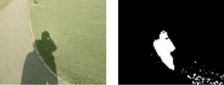
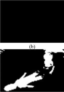
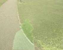
Fig. 4 shows the shadow detection results for “Field.jpg” using algorithm B. In Fig. 4(b), it is observed that upper half portion of the shadow region is detected while in Fig. 4(c) lower half portion of the shadow region is detected. Lastly in Fig. 4(d) whole shadow region is detected when thresholding of L channel only is used.

The results of shadow detection for “Girl.jpg” using Algorithm B are shown in Fig. 5. As shown in Fig. 5(c), the girl in the original image is no longer misclassified as shadow when thresholding of both L channel and b channel is carried out. Again it shows that when thresholding of both L channel and b channel works especially well for shadow region under yellow-colored background.

(a)

(c)

(d)

Fig.5. Experimental results for shadow detection using Algorithm B. (a) Original image. (b) Shadow mask obtained via thresholding of both L and a channel. (c) Shadow mask obtained via thresholding of both L and b channel. (d) Shadow mask obtained via thresholding of L channel only.

• C.    Comparison of Results

(a)

(c)

(d)

From Fig. 6, Algorithm B identified shadow of the flag pole precisely while both method by [15] and Algorithm A misclassified great area of non-shadow region. Therefore Algorithm A has the highest accuracy in shadow detection. Comparing all algorithms in terms of shadow removal, both Algorithm A and Algorithm B have better estimation in color of replaced flag pole shadow compared to method by [15].

(a)

(c)

(d)

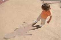
From Fig. 7, it is observed that method by [15] and Algorithm A are more likely to misclassify object as shadow region compared to Algorithm B. Method by [15] and Algorithm A has detected the object wrongly and increase its intensity.

Elapsed processing time (based on Matlab R2014a) for all implemented algorithms for each result image counted in unit of second are tabulated in Table 1. From Table 1, we can conclude that in terms of elapsed processing time, overall Algorithm B has the shortest processing time, followed by method by [15] and lastly Algorithm A. As method by [15] and Algorithm A tend to misclassify object as shadow region, such mistake would result in more workload for shadow removal and hence unnecessarily costing more processing time compared to Algorithm B.

Table 1. Processing Time Required for All Implemented Algorithms

Algorithms	“Field.jpg”	“Girl.jpg”
Method by [15]	4.241 sec	2.142 sec
A	6.792 sec	2.345 sec
B	3.409 sec	1.820 sec

• V.    Conclusion

This work presents two shadow removal algorithms named Algorithm A and Algorithm B. Algorithm A involves exploitation of illumination and color information of RGB image while Algorithm B is executed based on approach of applying thresholding on Lab color space channel. These proposed methods are compared against method developed by [15]. In conclusion, Algorithm B has successfully achieved the major objective as it has achieved requirement of adequately accurate shadow detection and short processing time.

Misclassification of less illuminated or dark objects as shadow region often causes complication in achieving objective of achieving high accuracy for shadow detection algorithm. Unlike method by [15] and Algorithm A, Algorithm B applies thresholding on all three color channels of Lab color space instead of utilizing illumination information gained from L channel only. This approach successfully deals with misclassification problem of dark objects. Through comparison of results from all algorithm, Algorithm B has the best performance in terms of shadow detection accuracy. However, Algorithm B requires careful selection of thresholding method to fully utilize its capability to identify shadow region from a single color image accurately.

Quantitative analysis has been done on image intensity profiles for result images from all implemented algorithms. Algorithm B shows highest effectiveness in reducing shadow effect. Algorithm B has better estimation on the color to replace detected shadow region as compared to other algorithms. Compared to the method by [15] and Algorithm A, Algorithm B has the lowest processing time measured in unit of second as it has less computational workload due to its higher accuracy in shadow detection.

Acknowledgment

The authors would like to thank the reviewers for their constructive comments. This work was supported in part by the Universiti Sains Malaysia’s Research University Individual (RUI) Grant with account no. 1001/PELECT/814169.