Development of growth poles in the Russian Federation: direct and reverse effects

The issues of spatial development management are of special interest for the Russian Federation the area of which is of considerable scope, and the characteristics of its individual territorial units are rather diverse. The importance of socio-economic space transformation is enhanced under the conditions of increasing interregional differentiation in a number of key indicators (for example, the difference between the maximum and minimum values of per capita GRP in the period from1998 to 2017 has increased from 20 to 54.8 times1): significant regional disparities distort space being evidence of its integrity lack.

Meanwhile, a single coherent space, the importance of which was emphasized by E.G. Animitsa, N.M. Surnina [1], E.M. Bukhval’d [2], A.I. Tatarkin [3] and other authors in their studies, may not be homogeneous: each territory has its own set of strengths and weaknesses determining the nature and efficiency of socioeconomic processes within its borders, making the attempts to influence specific regions and municipal entities in an effort to align their development parameters costly and ineffective. Thus, according to N.V. Zubarevich [4] there is a need to address significant contradictions only between the social characteristics of the territories’ development (while smoothing spatial economic inequality due to its being conditioned by the objective factors is impossible).

Moreover, within the concept of polarized development dominating in the regional policy carried out at the present time in Russia 2, advancing the development of certain territorial elements is perceived as a source of positive transformation of large territorial systems.

The basis of this concept is the theory of cumulative causation of G. Myrdal [5] who noted close dependencies between all the parameters of the system development; its change consequently determines the impulses transmitted by the individual system elements. Obviously, in this case national and regional development are rather divergent than convergent in nature, and a key factor is the formation of the economic leaders being the agents of positive transformation. The term “growth poles” was proposed by a French scientist F. Perroux [6] who identified them as compactly arranged and dynamically developing sectors or individual companies concentrating a “momentum of development”, influencing the territorial structure of the economy and its dynamics. He also stressed the objective nature of their formation: all economic actors are initially different from each other, and the magnitude of these differences over time, only increase. F. Perroux’s ideas were continued in the studies of another French economist, J. Boudeville [7], he not only outlined the conditions of the growth points emergence, but also offered to understand them as the territory of different scales which are the sources of innovation and economic development across the country together with enterprises and industries. The approach of F. Perroux and J. Boudeville gained quality development in the works of P. Pottier [8] who suggested that spaces connecting individual growth poles and serving as the sites for infrastructure networks, develop more intensively than other areas, becoming over time, the corridors (or axes) of development and turning into the elements of spatial framework for the country’s economic growth.

In turn, the transformation of the territories that do not fall in the number of poles or axes of growth, is determined by their interaction with the leaders. Thus, T. Hagerstrand [9] considered the diffusion of innovations as the basis for synchronizing the pace of development of the regions different from one another: capital seeks from development centers to peripheral areas where resources are more accessible, thereby causing their economies to grow. This approach is reflected in the “volcano” model of H. Hirsch [10], according to which the growth pole periodically provides impulses of innovations to the surrounding territories, as a result the periphery gains access to innovations, gradually increasing its level of well-being and getting the opportunity of becoming a center of development.

Over time, the interest of researchers considering the factors of territories’ transformation into growth poles has shifted to studying the opportunities of agglomeration development and the evaluation of agglomerations’ role in the country’s conversion (primarily the economic one): the “centerperiphery” theory of J. Friedman [11], the works of H. Richardson [12] and P. Romer [13], devoted to agglomeration effects, the concept of new economic geography of M. Fujita, P. Krugman and E. Venables [14], the theory of clusters by M. Porter [15] deserve special attention.

In the modern foreign studies the issues of heterogeneity of various territories’ development also receive much attention; the authors of the research works emphasize both the difficulty of overcoming the backlog of economically weak regions and cities from the leaders [16; 17; 18; 19], and the prospects opening to the space systems the formation and development of growth poles – agglomerations, clusters [20; 21; 22]. These topics are quite popular among the Russian authors [23; 24; 25; 26], especially because the process of studying the issues of transformation of the spatial organization of the economy has a long history in domestic science (so, clusters [27] corresponding to the models of growth poles in a number of characteristics were the basis for the Soviet model of productive forces).

Such a “bilateral” approach to the prioritization of spatial transformations (on the one hand, the desire to remove a significant interterritorial imbalances, on the other hand, the formation and support of growth poles) seems contradictory, but these priorities can be combined with each other within the framework of the concept of polarized development (but only in case, if the imbalances elimination does not mean the complete removal of the differences between territories). Moreover, in theory the growth poles are able to act as an effective instrument for reducing the level of interregional differentiation (think of the model of T. Hagerstrand, H. Hirsch), that determines the emergence of a considerable number of works in the scientific literature based on the search of possibilities of applying the concept of polarized development in today’s conditions [28; 29]. Despite the fact that the theory of growth poles has not lost its popularity nowadays, some researchers’ evaluation of the capacity and efficiency of the implementation of the polarized development concept in practice is somewhat controversial. For example, S.E. Dronov notes that the accelerated development of the two capitals (Moscow and Saint Petersburg) has not secured their becoming the points of growth, promoting the economic development of the surrounding areas, moreover, it has led to the increased inequality between them [30], G.F. Shaikhutdinova describes the development orientation of the individual elements of the space leading to the buildup of uneven socioeconomic development of territories as the main drawback of the concept of growth poles [31, p. 40]. Indeed, the advanced development of territories which could become the economy growth points of both the country as a whole and of the individual regions and municipalities (especially those located close to them), often leads to the reverse effect: inter-territorial contrasts are only aggravated.

At the same time in the works mentioning the presence of such (direct and reverse) effects of polarized development, only the fact of their manifestation is emphasized in most cases, and the authors concentrate either on the use of benefits in the process of growth poles allocation, or in the designation of causes and consequences of the imbalances conditioned by the rapid development of economic leaders. The scale of the impact (positive or negative) they exert on the territories concentrated around them is left without proper attention. All of the above determined the choice of the study objective which is to develop an approach for assessing the impact of the growth poles on the surrounding space.

Description of the research methodology and the justification of its choice

The analysis of spatial characteristics of the socio-economic systems cannot rely only on the assessment of the extent and dynamics of individual development indicators, although it does not exclude it: the priority is the consideration of the objects’ (and their aggregates’) location features in the space; and the parameters of the objects proximity of to each other, their concentration in the territory, the scale of their systems become important aspects for the research.

Obviously, the simplest method of spatial development features analysis is the interterritorial comparison of the values of the considered indicators (e.g., the identification of the ratio of the maximum and minimum values of the studied parameter, the definition of the Gini coefficient which allows to characterize the degree of differentiation of separate space elements development, etc.). The result of such comparisons is the definition of the parameters of spatial development heterogeneity which allows us to make generalized conclusions about the extent of polarization of the economy (or social sphere), but does not give a full picture of the degree of dependence between the development parameters of the more successful territories and their neighbors (interterritorial comparison allows only to ascertain the presence or absence of failures).

Considering agglomerations (compact clusters of settlements closely connected by the economic and social flows, and implementing the effects of localization and concentration, the effects of scale of production through the interaction with each other [32]) as potential growth points provides researchers with the ability to use the whole complex of parameters to assess the extent of their development: the coefficient of agglomerations, the index of agglomerations, the coefficient of agglomeration population’s development [33], etc. However, this approach allows you to focus on the growth points (and the place occupied by them in the socio-economic system of a region or country), failing to take into account the features of transformations of the territories surrounding them.

In turn, to identify the degree of connectedness of the individual space components with each other the evaluation of spatial autocorrelation can be used, which can be defined as follows: for a set S containing n geographical units, spatial autocorrelation is a correlation between the variable observed in each of the n units, and the measure of geographical proximity defined for all n ( n -1) pairs of items from S [34]. Thus, the analysis of spatial autocorrelation allows you to set the tightness of the relationship between the parameters characterizing the development of the territories located near to each other.

One of the most common (and easy to use) parameters of spatial autocorrelation assessment is the Moran’s I index, which is presented as a methodological basis of a number of foreign studies [35; 36; 37]. Assessment of the Moran’s I index involves the following steps.

The first step includes building a distance matrix containing information about the distances between all the studied territorial units (in this research, Russian regions). There are various approaches to determining values for the matrix: for example, they can be assumed as equal to zero (if the territories do not have a common border) or unit (if such a boundary exists), they can be determined based on the information about the distance in the air, on the length of roads or railway lines between the considered areas.

In the framework of this research the distance matrix was built based on the information on length of roads between administrative centers of the subjects of the Russian Federation.

The second step includes calculating the value of the global Moran’s I index and determining the presence (or absence) of spatial autocorrelation.

The formula for calculating the global Moran’s I index (1) is as follows:

I = n Z ” = , Z n = i wAx - x ⁾⁽ x

- x )

,

⁵ 0 Z n _{= 1}( x i - x ⁾²

where I is the global Moran’s I index, x is the indicator, S₀ is the sum of all spatial weights ( S₀ = ∑ _{i =1} ∑ _{j =1}w _ij ), n is the number of the analyzed areas.

The index values can lie in the range from -1 to 1, and its comparison with the mathematical expectation (2) allows to make a conclusion about the presence and nature of spatial autocorrelation .

E ( I ) = — , n - 1

where E(I) is the mathematical expectation of the index, n is the number of the analyzed areas.

The obtained values can be interpreted in the following way. If the value of the Moran’s I index exceeds the mathematical expectation, there is positive spatial autocorrelation (observation values in the adjacent territories are close to each other); if the mathematical expectation exceeds the value of the Moran’s I index, we can confirm the presence of negative spatial autocorrelation (the values of the considered indicator of the territories located near each other differ). If the Moran’s I index has the same value with the mathematical expectation, it indicates no spatial autocorrelation [38].

Testing the significance of the obtained results can be carried out using the traditional econometric method of statistical testing of hypotheses (z-test), which is carried out by determining the value of Z-statistics (3) .

I - E ( I )

z - statistics = ,              ,     (3)

4E ( 1 ²) - E ( I ) ^{2 ,}        '

where I is the global Moran’s I index, E(I) is the mathematical expectation of the index.

This value shows how many standard deviations the actual value of the Moran’s I index is removed from the expected value. The higher is the value, the less likely it is that the actual pattern is random.

The third step is the calculation of the values of local Moran’s I index and the determination of the closeness of the relationship between the individual territories.

The local Moran’s I index allows to identify the presence and nature of the relationship of a particular territory with all the others [39]. The calculation of its value may be carried out using the formula (4):

IL,= zi ^ w y z j , (4)

where I _L is the local Moran’s index for the i-th territory, w_ij is a standardized distance between the i-th and j-th territories, z_i and z_j is the standardized values of the studied parameter for the i-th and j-th territories.

The obtained values can vary from -1 to 1, and the logic of their interpretation coincides with the logic of the evaluation the values of the global Moran’s I index.

Separate parts of the local index (5), the values of which characterize the strength of interaction between two specific territories may also be of interest :

LISA_ij = z_iz_jw_ij , (5)

where LISA_ij is the force of interaction between the i-th and j-th territories, w_ij is a standardized distance between the i-th and j-th territories, z_i and z_j is the standardized values of the studied parameter for the i-th and j-th territories.

The fourth step involves the grouping of the territories in accordance with the ratio of characteristic standardized values of the considered indicator and the values of spatial factor (which allows us to determine the place of each territorial unit in the spatial system, identify its leaders, extreme points and the peripheral area, to implement spatial clustering).

If you combine the standardized values of the estimated measure (z) with its spatially weighted centered values (wz) for each of the analyzed territory in the same coordinate system, we can see that the points (describing the territorial units) are localized in one of four quadrants [40].

For the territories characterized by relatively high values of the considered indicator and neighboring the territories having similar values of the considered parameter, the values of z and wzwill be positive (HH quadrant – extremums). Negative values of z and wz (LL quadrant) indicate that the territories are located close to the entities similar in magnitude of the analyzed sector, and the value of the considered parameter is relatively low. If the value z is positive and wz is negative (HL quadrant), the territory differs from its neighbors being ahead of them by the estimated parameter. If, on the contrary, z is negative and wz is greater than zero (LH quadrant), the territory is behind its neighbors. Thus, the territories with positive autocorrelation fall within the HH and LL quadrants, if the autocorrelation is negative, they fall within HL and LH quadrants. To visualize the outcomes of the calculations better it is possible to use the cartographic methods of representation helping to render the clusters of the subjects of the Russian Federation which have fallen into different groups (quadrants) as well as to highlight the regions influencing each other most strongly.

Thus, the evaluation of spatial autocorrelation allows not only to identify the interrelationship between the individual territories, but also to measure it, identify the leaders (not only by development scale but also from the point of view of the strength of their impact on neighbors) and the outsiders. Based on the “classic” conception of the growth poles nature (suggested in the interpretations of F. Perroux and J. Boudeville), it can be assumed that their key characteristics are, on the one hand, the high level of development that allows them to stand out among other subjects, on the other hand, the importance of their impact on the development of other socio-economic systems (the entire socio-economic system as a whole). In the context of the above approach to the territories grouping (based on the calculations of the Moran’s I index) the potential growth poles are the entities within HH and HL groups (they are characterized by quite high values of the considered indicators) and having substantial values of the local Moran’s I index ( IL ) at the same time, indicating a close relationship between their development and the development of other territories. In this regard, it makes sense to divide each group of the regions allocated in the framework of further analysis into two parts (in accordance with the parameters of the local Moran’s I index these are the territories that get into it, the regions which are most closely related to other entities are of particular interest), although this division is not always possible in practice (there may be a situation when there will be no regions the development of which is significantly associated with the development of other participants in the economic system within the group).

The results of the study, analysis and explanation

In order to determine how growth poles effect on the surrounding space, such figures as “permanent population” and “gross regional product” were analyzed3. Their choice is dictated by the fact that both indicators can be considered as a result parameter of the territory’s development. Thus, the value of the gross regional product shows the scale of economic activity carried out in the region, and will depend on the success of its implementation. In turn, the distribution of population in the country space is a consequence of the aggregate of complex demographic and socio-economic processes and patterns largely determined by the success of individual territorial systems development.

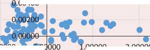
Assessment of spatial autocorrelation conducted on the basis of the analysis of data on the population in the Russian regions, suggests a direct connection between the values of this indicator in the territories close to each other. Such conclusions are possible due to the comparison of the values of the global Moran’s I index (0,020) calculated using the formula (1) with its mathematical expectation (-0,012), to determine which the formula (2) was used. This means that changing the value of the examined indicator (the population) in the transition from region to region is gradual. While the two “leaders”, the growth poles are clearly observed (Moscow and the Moscow Oblast), which are not only characterized by high population, but also have a significant impact on the surrounding regions: the points representing them are much to the right of the main array ( Fig. 1 ).

The largest share in the total number of the regions is occupied by the territories with negative autocorrelation (LH group) – with low values of the considered indicator surrounded by territories where the population is relatively high ( Tab. 1 ). Almost all the regions included in this group and is characterized by strong intra-regional links are located close to Moscow (and Moscow Oblast).

Extremums are the regions in HL group having a significant value of the considered indicator (compared to the neighboring regions), characterized by very low values of the local Moran’s I index so that we could speak about a significant impact on the surrounding territory on their part.

Another group of the regions having relatively high population values (but differing by positive autocorrelation) is HH group. These are the territories comparable with the sur-

Figure 1. Spatial Moran scatterplot for subjects of the Russian Federation (the permanent population)

WZ

0.01400

0.01200

Ryazan Oblast

0.01000

-2.00000

0.00800

0.00600

3.00000

-1.0000-00.002000.00

2.00000

-0.00400

-0.00600

Moscow Oblast

4.00000

5.00000

Moscow

6.00000

Z 7.00000

Based on: Regions of Russia. Socio-economic indicators. 2018: stat. coll. Rosstat. Moscow, 2018. Pp. 39-42.

rounding regions by the values of the considered indicator. They represent the elements of the area of the country’s population concentration. The maximum values of the local Moran’s I index are characteristic for the representatives of this very group, Moscow and the Moscow Oblast (already noted earlier). However, it should be noted that positive values of the index for these territories are related to their proximity to each other (with a substantial population in each of the regions), whereas the relationship with the surrounding territories is reverse.

LL group (the regions not experiencing the influence from the subjects surrounding them which are the objects of the study, and are not the leaders either) includes mainly the Far East and southern part of the country.

The calculations (and also the graphic display of the regions’ grouping in accordance with their role in the national settlement system, presented at Fig. 2) indicate the presence of correlation between the indicators of the population residing in the neighboring territories. At the same time, the analysis of the closeness of the relationships (within the given parameters) between the regions shows that only the impact of the complex including Moscow and the Moscow Oblast on the surrounding territories can be called significant.

Meanwhile all connections linking Moscow with the regions belonging to the area of significant impact of the leading territories, and shown with lines in Fig. 2 are reversed. This means that capacity building of Moscow (and the Moscow Oblast) in the long run will not lead to amplification of the related regions (located around the Moscow Oblast), on the contrary, it will result in an outflow of resources available to them.

The validity of this thesis is also confirmed by a retrospective analysis: the evaluation of population change in the Russian regions over a sufficiently long period (60 years) indicate that the regions located in the European part of the country neighboring the Moscow Oblast are leading in the pace of population decline: some of them lost more than a third of their

Table 1. Groups of subjects of the Russian Federation, having different positions in the national settlement system*

The subject of the Russian Federation ILi The subject of the Russian Federation ILi LH HH Ryazan Oblast -0.0040 Moscow Oblast 0.0221 Kaluga Oblast -0.0027 Moscow 0.0143 Republic of Adygea -0.0027 Nizhny Novgorod Oblast 0.0023 Novgorod Oblast -0.0020 Sverdlovsk Oblast 0.0021 Tver Oblast -0.0018 Republic of Bashkortostan 0.0021 Republic of Mari El -0.0016 Rostov Oblast 0.0017 Kostroma Oblast -0.0015 Chelyabinsk Oblast 0.0017 Oryol Oblast -0.0014 Saint Petersburg 0.0015 Vladimir Oblast -0.0014 Samara Oblast 0.0013 Tambov Oblast -0.0013 Republic of Tatarstan 0.0009 Ivanovo Oblast -0.0013 Perm Krai 0.0008 Republic of Mordovia -0.0012 Saratov Oblast 0.0006 Republic of Kalmykia -0.0012 Volgograd Oblast 0.0005 Smolensk Oblast -0.0011 Voronezh Oblast 0.0005 Pskov Oblast -0.0011 Leningrad Oblast 0.0003 Lipetsk Oblast -0.0011 Orenburg Oblast 0.0002 Tula Oblast -0.0010 Novosibirsk Oblast 0.0002 Kurgan Oblast -0.0010 Omsk Oblast 0.0001 Sevastopol -0.0009 Kemerovo Oblast 0.0001 Karachay-Cherkess Republic -0.0008 Altai Krai 0.0000 Other subjects of the Russian Federation LL HL Republic of North Ossetia-Alania 0.0027 Krasnodar Krai -0.0008 Republic of Ingushetia 0.0027 Republic of Dagestan -0.0005 Kabardino-Balkar Republic 0.0006 Stavropol Krai -0.0003 Jewish Autonomous Oblast 0.0006 Krasnoyarsk Krai -0.0001 Amur Oblast 0.0003 Irkutsk Oblast -0.0001 Magadan Oblast 0.0003 Republic of Crimea -0.0001 Khabarovsk Krai 0.0003 Primorsky Krai 0.0000 Sakhalin Oblast 0.0002 Chechen Republic 0.0002 Chukotka Autonomous Okrug 0.0002 Republic of Sakha (Yakutia) 0.0001 Zabaykalsky Krai 0.0001 Kamchatka Krai 0.0001 Republic of Buryatia 0.0000 * In bold italics are the subjects of the Russian Federation having strong inter-territorial links with the surrounding territories (the value of the local Moran’s I index for them taken modulo exceeds the modulus of the average value of the calculated local Moran’s I indices). Based on: Regions of Russia. Socio-economic indicators. 2018: stat. coll. Rosstat. Moscow, 2018. Pp. 39-42. human resources during the period under review (Tab. 2). The extent of population reduction in the central part of the country in the long term is not inferior to the parameters of the existing human capital loss in the Far East territories the global nature of which much is described in the scientific literature [41; 42].

It is obvious that the currently observed processes of socio-economic space “contraction” to single points referred to by such researchers as A.I. Tatarkin [3] and N.V. Zubarevich [43] are characteristic not only for the Central part of the country. However, the Moscow region’s role in these processes is the most significant: in recent

Figure 2. The influence of the subjects of the Russian Federation on each other (indicator – resident population)

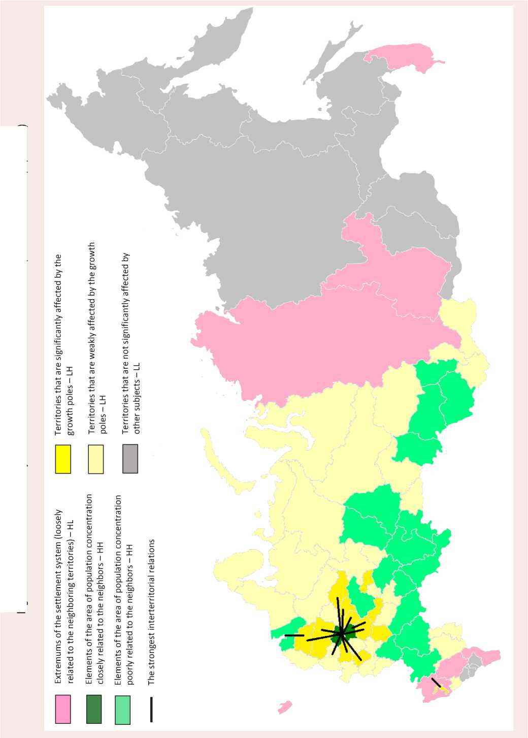
Table 2. The regions with the highest rates of population decline*

No.	The subject of the Russian Federation	Population, thousand people		Population decline rate, %
		1959	2019
1.	Tambov Oblast	1549	1016	34.41
2.	Pskov Oblast	953	630	33.93
3.	Kirov Oblast	1886	1272	32.55
4.	Kostroma Oblast	921	637	30.81
5.	Tver Oblast	1805	1270	29.66
6.	Kursk Oblast	1483	1107	25.35
7.	Magadan Oblast	189	141	25.27
8.	Sakhalin Oblast	649	490	24.56
9.	Tula Oblast	1918	1492	22.90
10.	Ryazan Oblast	1445	1122	22.89
11.	Bryansk Oblast	1550	1211	22.57
12.	Ivanovo Oblast	1288	1015	22.04

* In bold italics are the subjects of the Russian Federation, bordering the Moscow Oblast or located close to it.

Based on: Demographic Yearbook of Russia. 2002: stat. collection. Goskomstat of Russia. Moscow, 2002. Pp. 22-24; Federal state statistics service. URL: (date accessed: 24.10.2019).

decades, a steady increase in the proportion of people living in 15 major cities is recorded, while the total number of their inhabitants for the period from 1989 to 2018 increased by 16%, the number of inhabitants living in Moscow increased by almost 40% for the same period4. As noted in the researches of Zh.A. Zaionchkovskaya and G.V. Ioffe, since 1960 migration has been the main growth driver of the population of Moscow and the Moscow Oblast (even though its actual magnitude exceeds the officially recorded numbers) [44]. It should also be noted that, according to experts-demographers, “the attraction of large Moscow and the Moscow Oblast extends to the whole CIS region, but despite this their migration gain three-quarter consists of the arrivals from the Russian regions up to the Far East” [45].

At the same time the greatest strength of attraction of Moscow and the Moscow region is felt by the nearby entities. According to the results of a study conducted by Strelka Mag editorial board (issued by the Institute for media, architecture and design “Strelka” specializing in urbanism and urban development) together with the Socialdatahub company, the rating of Russian cities the residents of which often move to Moscow was built5. It was headed by Saint Petersburg, Yekaterinburg and Nizhny Novgorod, and Ryazan and Tula located near the Moscow region though entered the Top 20, only took 16 and 19 places, respectively. However, if you count the values used to rank municipalities that characterize the number of residents who moved to Moscow in the relative form (specifying their ratio to the total number of people living in these cities), we can see that the performance of Ryazan (4%) and Tula (3.6%) is higher than parameters of Saint Petersburg (3.1%), Yekaterinburg (2.9%) and Nizhny Novgorod (3.2%).

The parameters of spatial autocorrelation, identified on the basis of estimates of gross regional product, are somewhat different from the previously defined characteristics of the tightness of the relationship between the values of the “permanent population” indicator inherent in the considered subjects of the RF. The value of the global Moran’s I index (-0.001) is less than its mathematical expectation, which allows to conclude that a negative autocorrelation (the outcomes of z-test confirm the significance of the results). This means that changing the values of the considered parameter when moving between the regions occurs “abruptly”, and the difference between the volume of GRP of neighboring territories is typically quite substantial.

At the same time there is a lot in common between the spatial distributions of population and the amounts of the produced product. Thus, strong leaders on the value of the evaluated indicator having the closest ties with their neighbors are again Moscow and the Moscow Oblast (Fig. 3), and the territories surrounding them lead in LH group (the regions which are characterized by negative autocorrelation and low values of GRP).

However, high values of the local Moran’s I index are characteristic only for the 19 subjects of the Russian Federation ( Tab. 3 ), which means that they have strong enough relationships with the neighboring regions. The leaders among them (on the value of the considered indicator) along with the already noted earlier are Saint Petersburg and Krasnodar Krai (however, the extent of the closeness of their relationship with the surrounding territories significantly inferior to the parameters of connectedness of Moscow (and the Moscow Oblast) with the neighboring regions).

Analysis of locations of the regions in different groups (HH, HL, LH, LL) in the country ( Fig. 4 and 5 ) attests to the high degree

Figure 3. Spatial scattering diagram of the Moran’s I index for the subjects of the Russian Federation (gross regional product)

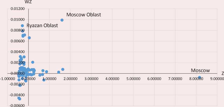
Based on: Regions of Russia. Socio-economic indicators. 2018: stat. coll. Rosstat. Moscow, 2018. Pp. 458-459.

Table 3. Groups of subjects of the Russian Federation allocated in accordance with the parameters of spatial autocorrelation (indicator – gross regional product)*

The subject of the Russian Federation ILi The subject of the Russian Federation ILi LH HH Ryazan Oblast -0.0026 Moscow Oblast 0.0159 Tver Oblast -0.0022 Saint Petersburg 0.0012 Kaluga Oblast -0.0019 Vladimir Oblast -0.0018 Tula Oblast -0.0013 Ivanovo Oblast -0.0012 Kostroma Oblast -0.0010 Novgorod Oblast -0.0010 Smolensk Oblast -0.0009 Oryol Oblast -0.0008 Pskov Oblast -0.0007 LL HL Republic of Ingushetia 0.0021 Moscow -0.0060 Republic of North Ossetia-Alania 0.0020 Krasnodar Krai -0.0009 Kabardino-Balkar Republic 0.0009 Chechen Republic 0.0009 * The table presents only those subjects of the Russian Federation, which have the most strong interterritorial ties with the surrounding territories (their values of the local Moran’s I index taken modulo exceeds the modulus of the average value of the calculated local Moran’s I indices). Based on: Regions of Russia. Socio-economic indicators. 2018: stat. coll. Rosstat. Moscow, 2018. Pp. 458-459. of polarization of economic activity in the European part of Russia. The obtained results can be interpreted as follows.

Most of the Siberia regions although characterized by highly significant values of the considered indicator, are poorly connected with the surrounding territories (this is largely due to the significant distances between the centers of economic activity of these subjects of the Russian Federation). The Far East and parts of Southern Russia do not experience a significant impact from their neighbors (the near-border location of these regions causes the need for analysis of the extent of their relationship with the neighboring foreign countries and regions as it is possible that they may fall within the zone of influence of the economic development extremums beyond the borders of the Russian Federation), and the Ural regions characterized by quite high values of GRP (mainly autonomous district) have (within the framework of the considered parameter) closer relationship with Moscow than with each other (as evidenced by the results of the calculations of LISAij indicators values defined for the regions of the Urals and Moscow). This regularity is confirmed by the results of the analysis of statistical data characterizing the interregional trade flow. Thus, the trade turnover of the Tyumen Oblast (including Khanty-Mansi and Yamalo-Nenets Autonomous okrugs) with Moscow is more than 4 times greater than trade with the Sverdlovsk Oblast, more than 10 times with the Chelyabinsk Oblast, more than 160 times with the Kurgan Oblast6. Moscow also takes leading position in the structure of the interregional trade turnover of the Chelyabinsk Oblast (although the share of the Sverdlovsk Oblast

Figure 4. The influence of the subjects of the Russian Federation on each other (indicator – gross regional product; direct inter-territorial ties are displayed)

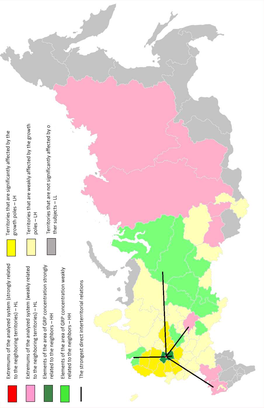
Figure 5. The influence of subjects of the Russian Federation on each other (indicator – gross regional product; reverse inter-territorial ties are displayed)

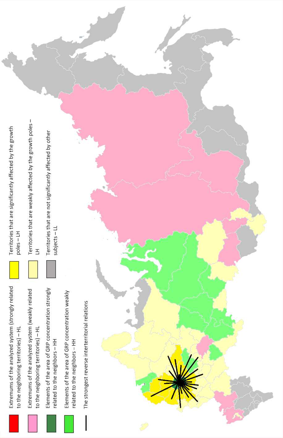
and Yamalo-Nenets Autonomous Okrug is quite high) [46, p. 839]. A bit different situation has developed in the Sverdlovsk Oblast: A.A.Glumov in his study of economic relations of the Ural territories notes [47] that the Chelyabinsk Oblast is ahead of Moscow in terms of trade turnover size with the region; moreover, if you combine the statistics on the South of the Tyumen Oblast and the autonomous districts constituting it, Moscow will take only third place in the resulting structure of trade and economic relations of the Sverdlovsk Oblast. At the same time, the “gravity” of the Urals Northern territories to the administrative center of the country is not in doubt: the similarity of economies scale and the prospect of markets determines the high interest of the territories in each other. It’s no coincidence that an approach whereby not a geographical, but an “organized” proximity (based on the similarities, the belonging to a single relations system) gains special attention when determining the prospects of the subjects’ successful cooperation, gets spread in the scientific literature [48]. In turn, the entities considering the neighboring regions as potential markets for manufactured products recognize that the level of inter-territorial cooperation between the Ural regions is not high enough; this factor leads to the activation of their attempts to strengthen interregional integration: in 2019, at the initiative of the representatives of the industrial complex of the Urals Federal district the Expert Council of the UrFD7 was formed to facilitate the development of cooperation between the territories of the district and to bring business, power structures and scientific community together.

Continuing the explanation of the results received in the course of the study it should be noted that the strongest direct interregional ties of the economic leader (Moscow) with other areas are “remote” in nature: the regions directly affected by the growth pole’s development are separated geographically from them (the only exception is the Moscow Oblast). The subjects of the Russian Federation located near the Moscow region are also under its significant influence, but the nature of the observed relationships (see Fig. 5 ) does not allow to conclude about the presence of direct relation between their economic development. At the same time the presence of strong reverse interterritorial relations with Moscow is characteristic for all territories “girdling” the Moscow region.

Conclusion

The methodological approach used in the research certainly has its limitations (it allows to identify the relationship between the territories on the basis of only their locations and magnitude values of the considered index), besides, only two variables were analyzed in this research. Consideration of additional parameters, as well as the change in the study scope (e.g., the transition to the municipal level) would allow to reveal a greater number of patterns, to identify other growth poles and clusters (however, it should be noted that the process of identifying development centers and assessing their prospects is extremely challenging and cannot only be based on the method of spatial autocorrelation which was used as a methodological basis for this study). At the same time, the work done makes it possible to offer a few theses.

The impact of territorial leaders, growth poles, on the surrounding space can be very ambiguous. The calculations have proved that the proximity to the advanced socio-economic systems that (in accordance with the theory of diffusion of innovation) should generate pulses of development to their neighbors not only deprives the regions of significant advantages, but also causes the large-scale outflow of resources only exacerbating the existing problems. Dynamic conversion of growth poles determines the need for a significant amount of additional resources coming from the outside (close neighbors are primarily the source of these resources). This allows a critical approach to some aspects of the theories of polarized development and diffusions of innovation: one cannot argue that the emergence in the socioeconomic environment of the subjects leading in their development the surroundings and stimulating economic growth of large-scale systems (e.g. the national economy) will have a positive impact on all elements of the economic complex, their effects on the immediate neighbors will be rather negative.

In this regard the simultaneous solution of such problems of the spatial development Strategy of the Russian Federation for the period up to 2025 as “reduction of regional disparities in socio-economic development of the subjects of the Russian Federation, and also reduction of intra-regional socio-economic disparities” and “ensuring the expansion of the geography and economic growth, scientific-technological and inno-vative development of the Russian Federation due to socio-economic development of the most promising centers of economic growth”, is quite a challenging task. This does not mean that the territories surrounding the capitals, the administrative centers and the leaders of economic development are to be doomed. Rather, we should consider that the formation of (development support) growth poles is not a universal remedy the use of which would provide the solution to all problems, and the territories adjacent to the leaders need special attention when implementing the polarization of the economy. Development of priorities and mechanisms for balanced regional policies that would take into account both the interests of the national economy and possibilities of transformation of the territories adjacent to growth points is a promising topic for further research.