Development of launch vehicle control algorithm for the initial part of the trajectory using the ACOR method

Introduction. At the initial stage of the launch vehicle (LV) flight at altitudes between 200–300 meters one of the flight control system’s tasks is to displace the launch vehicle’s jet engine flame from the launch complex (LC). This process is of great importance as the jet engine flame has a negative impact on the LC [1].

There are several methods to reduce negative thermal effect on LC. Some of them are:

• 1.    Methods of “passive” protection: to use heatproof materials in the constructions of the LC or to use additional measures such as foam or water to cool the launching complex elements [2; 3].

• 2.    To use some modified algorithms of a LV flight control to displace LV jet flame in specially organized direction and so on.

For example, at the LV of ground start “ZENIT” to cool jet engine flame and to protect LC facilities water is used [2]. While at the LV of sea launch “ZENIT-3SL” the technology of jet flame deviation to certain direction by means of modified algorithms of the LV flight control is used [4–6].

Two approaches can be proposed to perform controlled displacement of a LV trajectory using the vehicle flight control system (CS):

• 1.    Using pre-calculated motion program of a LV flight at the displacement phase (DP) taking into account initial and terminal (boundary) states of the vehicle and the subsequent executing of this program with use of the CS of the vehicle.

• 2.    Solving the synthesis problem of flight control taking into account the current and required terminal LV states.

In this paper we consider the second approach – synthesis of the LV fligth control algorithm. Solving the problem of jet engine flame displacement, the position of flame trace on the launch pad is one of output parameters of the LV flight control system.

To implement the controlled DP of the LV flight, the program of flame flow location on the launch pad in the direction of displacement l p ( h ) as a function the LV altitude h has to be preliminarily calculated. This program is fulfilled by the LV CS with flight control algorithm (regulator), specially developed for this phase of the LV flight.

In each time of DP the jet engine flame trace must be located inside a circular area of a certain size. The center of the area must be located on the line specifying the direction of the displacement. Size of the area has to be calculated in advance as a function of time for every particular LV and LC. Any high-rise structures should not be located in the direction of displacement.

Generally the model of LV motion at the initial phase of LV flight is described by nonlinear equations. But while solving the problem of LV jet flame displacement from launching complex constructions this model can be replaced by linearized equations with time variant parameters.

The problem of finding the optimal control of the system described by linear equations can be solved using the method of analytical construction of regulators (ACOR). The first scientific papers on this theme belong to A. M. Letov, published in 1960-s [7; 8]. In foreign publications this method is known as the tracking task method.

The aim of this work is to develop the method of construction of optimal regulator of a LV control system for the DP that provides the executing the program of jet flame trace displacement.

The problem is solved for linear equations describing the launch vehicle motion in the direction of displacement. The new modification of the ACOR method is proposed. The modified version of the method allows finding the solution of the problem when the system output is dependent explicitly on input variable.

Statement of the problem. While starting the LV nearest facility of the LC is the cable-filling tower. In order to prevent the LV collision with the tower the program of jet flame trace displacement on the launch pad as a function of trajectory altitude is used (fig. 1).

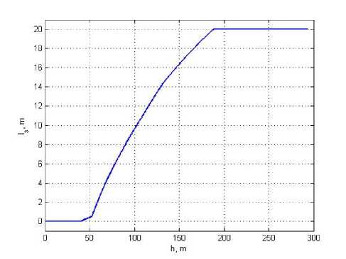
Fig. 1. Preset program changes the LV jet flame trace location as a function of flight altitude

Рис. 1. Заданная программа изменения положения следа оси ГД струи РН в зависимости от высоты полета

Double-stage character of this program is stipulated with the fact that after the lift-off the LV should move vertically to avoid hitting the cable-filling tower, then softly move in the direction of displacement on preset distance from starting point not setting engine plume close to the tower.

The control variable in the jet engine flame displacement problem is the engine nozzle deviation angle δ.

The task is to develop an optimal LV motion control law taking into account LV parameters and preset program of jet flame trace location at the launch pad, to choose the structure and gains of the LV CS regulator for executing the preset program of the jet flame trace displacement.

Efficiency of control is evaluated by quadratic terminal integral criteria. The terminal part of criteria is used to provide preset final angular state of the LV at the end of DP – vertical orientation and zero rate of LV. This requirement is caused by the fact that after completing the DP, the LV must continue its motion according to the regular pitch program. The integral part is some kind of a “penalty” for deviation of current output parameter l р from its preset program value l З [10].

The model of LV motion at the phase of controlled displacement. Parameters describing motion of the LV in the displacement plane are depicted in fig. 2.

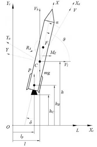
Fig. 2. Parameters of LV motion at the displacement phase in the starting frame

Рис. 2. Параметры движения РН на этапе увода в стартовой системе координат

Fig. 2 shows the main parameters of LV motion [11]: OL is the LV jet flame displacement direction, R A is the main vector of external forces, acting on LV, С is LV center of mass, F is LV pressure center.

Assumption:

• 1)    LV motion is performed in the plane of displacement maneuver;

• 2)    LV is considered as a solid body;

• 3)    the Earth gravitational field is homogeneous;

• 4)    the Earth is plain and nonrotating;

• 5)    atmospheric density during the DP is constant, wind disturbances are not considered;

• 6)    LV mass and inertia moments during the DP are constant;

• 7)    LV aerodynamic characteristics are: C x = const, C y = С Y ^α α , C d = const , where α – angle of attack; C x – aerodynamic drag force coefficient; C y – aerodynamic normal force coefficient; С_Y ^α – derivative of aerodynamic normal force coefficient; C_d – coefficient of pressure center;

• 8)    LV engine thrust during the DP is constant;

• 9)    the dynamics of engine thrust vector control actuator is neglected.

LV motion equation. Several reference frames are used in the article for description of LV motion (fig. 2): the starting frame OX C Y C Z C , the body frame CXYZ , the flow frame CX a Y a Z a [12]. The beginning O of starting frame is located in the crossing point of LV longitudinal axis, when LV is located on the launch pad (LP), with horizontal plane on zero level of launch pad. Axis OZ C form the right-handed frame OX_CY_CZ_C .

With enumerated assumptions the LV motion in the displacement maneuver plane is described by the following differential equations:

V h = ( P sin ( 9 +8 ) - mg - X a sin 9 + Y a cos 9 ) / m ,

V l = ( P cos ( 9 + 8 ) - Y a sin 9 - X a cos 9 ) / m ,

• <0 = (^- P sin ^{8 ( x}T ^{- x}B ) + Y a ⁽ x_d ^{- x}T ) ) / I ,         (1)

l=Vl, h= Vh,

ϑ=ω,

where m – LV mass; I – moment of inertia relative to lateral axis; V h и V l – projections of velocity V = V_h ² + V_l ² on flow axes h and l ; P – engine thrust; ϑ – pitch angle; θ= arctg ( V_hV_l ) – trajectory inclination angle; X_a = C_XS ρ V ² /2 – aerodynamic longitudinal force; Y a = C Y ^α α S ρ V 2 /2 – aerodynamic normal force, α =ϑ-θ ; h – LV center of mass (COG) flight altitude; l – distance from starting point to LV COG projection on the launch pad plane; ω – angular rate of LV relative to lateral axis; x T – distance from nozzle edge plane of sustainer engine to COG; x В – distance from nozzle edge plane to center of deviation of sustainer engine chamber; x d – distance from nozzle edge plane of sustainer engine to LV pressure center: x_d = L (1 - C_d ) ; L – characteristic length; S – characteristic area; ρ – atmospheric density; δ – angle of deviation of sustainer engine chamber; g – gravitational acceleration.

Simplifying and linearization of LV motion model. Considering values δ, α, Δϑ=ϑ-π /2, Δθ = θ-π /2 small, we will get:

sin ϑ≈ 1, cos ϑ ≈ -Δϑ , sin δ≈δ , cos δ≈ 1, sin ( ϑ+δ ) ≈ 1, cos ( ϑ+δ ) ≈-Δϑ-δ , V_h = V sin θ≈ V ,

V_l = V cos θ≈- V Δθ .

With these assumptions the system (1) transformed to the following two systems:

V^ = (p - mg - cxspV2/2) /m,         (2)

h i = V .

V₁ — ( - p A9 - P 5 - C Y S p V 2 a /2 + C X S p V ² A9 /2 ) / m ,

- ( h - ( X T - X B ) sin 9 ) ctg ( 9 + 5 ).

— V ,

(i) = ( - P 5 ( x_T - x_B ) + C Y a S ( x d - x , ) p V ² / 2 ) / 1 , a9 = to ,

where a — A9 -A9 , A6 = - Vl/V .

The system (3) can be rewritten in the following form:

V = (Cx - C)SpV2 -2p a9-CYaspVP l2

l = V ,

. = C(-x,>SpV2 a3+

2 I

Ca (Xd - x,) Sp V    P (X, - xB ).

-------------------V i ------------5 , A9 — ( .

2 I^l I

System (2) is independent from the system (4). It can be integrated with initial conditions: V(0) — 0 and

h(0) — h0 — XT to get explicit expressions for V and h as functions of time.

Several transformations of the first equation in the system (2) give the following results:

-”-V — 1 - C X ^p S V 2 ;

P - mg      2( P - mg )

m з     CpS a —--------, b —------------;

P - mg      2( P - mg )

2 adV aV — 1 -bV2, ^ ------— dt, ^

^J1 - bV^{2 J}

a

2 b

1 + 4ь v

1 - 4ь v

— t + c .

As V (0) = 0, so C = 0 and

V ( t ) — —j=th — t ;

ba h (t) — h + [Vdt — h + a ln ch — t. ba

One of system’s output parameter is the coordinate of jet flow trace l р along axis ОL .

Coordinates sustainer chamber center of deviations on the on the starting frame axes are described as follows:

l цк — l (x, Xb ) cos 9, hцк — h-(XT -XB)sin9.

Equation of the straight-line H = H ( L ), that goes through the sustainer chamber center of deviations and is parallel to thrust vector:

H - h цк — ( L - 1 цк )tg( 9 + 5 ).

Coordinate of jet flame trace on the starting plane can be evaluated with H = 0:

1p — 1 ЦК - hцкCtg (9 + 5), so

I — 1 -(XT -xb)cos9- n

At small angles 5 and A9 — 9 —

1_p — 1 + h ( A9 + 5 ) - ( X T - x b ) 5 .         (6)

So the final formula for calculation of output l р is:

1_p — 1 + h A9 + h_B 5 ,                 (7)

where h is the known function of time (5); h B = h – х T + х B – altitude of sustainer engine chamber center of deviation above the starting plane.

Preset coordinate of LV jet flow trace on the starting plane is denoted as l З ( h c ), where h c – altitude of nozzle edge plane of the sustainer engine above the starting plane.

h_c — h - x T .                     (8)

Formulas (5), (8) and l ₃( h_c ) can be used to recalculate the preset coordinate of LV jet flame trace along x axis as a function of flight time.

Motion equation of LV in vector-matrix form. System (4) can be written in normal Cauchy form:

—x ( t ) — A ( t ) x ( t ) + B ( t ) u ( t ),             (9)

dt

where x — [ V1 to 1 A9], is state vector; " a11 0 0 a14 ~ A — a 21 0 0 a 24 – dynamic matrix with elements 1 0 0 0 _ 0 1 0 0 _ a11 — -ca Sp V/2m, a14 — [(Cx - CY1) S p V2 - 2P]/2m, a2i — CY (xd - xT)Sp V / 21, a24 — CY (xd - x,) Sp V2 / 21;

B — [ b_; b₂ 0 0 ] ^, - vector with elements:

b 1 — - P / m , b ₂ — - P ( x , - x b )/ 1 ;

u = [δ] – control variable.

The system output vector is described by the algebraic equation:

y ( t ) — C ( t ) x ( t ) + D ( t ) u ( t ),             (10)

where y — [	V l	to	l p	T A9I - vector of output parame-
ters;	Г 1	0	0	0 "
	0	1	0	0
C —	0	0	1	h	; D — [ 0 0 h B 0 ] ' .
	. 0	0	0	1 _

Preset vector of output parameters is z — [ 0 0 1 з af.

Method of analytical construction of regulators (ACOR). Let’s consider linear time variable observable and controllable dynamic system (9); (10) with the initial conditions x(10) — x0 [9; 13]. In this system x(t) -n-dimensional state vector, u(t) – r-dimensional vector of control variables, y(t) – m-dimensional vector of outputs, z(t) – m-dimensional vector of demanded outputs.

Vector equation of tracking error at the time t is calculated as follows:

e ⁽ t ) = y ⁽ t ) ^- z ⁽ t ^).

It is necessary to find the control minimizing the criteria:

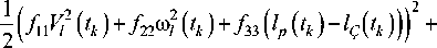
J (e, u) = 2 e (tk) Fe (tk) + tк                                               (11)

+ -J ( e T ( t ) Q ( t ) e ( t ) + u T ( t ) R ( t ) u ( t )) dt -2 t 0

In (11) F , R , Q – preset “weight” matrices, control variables u ( t ) are not constrained, t_k – preset final time.

It is shown [9; 13], that the solution of the problem if D = 0 gives to the optimal control law in the form:

u (t) = R-1( t) BT (t) [ g (t) - K (t) x (t)], where K(t) is n-dimensional quadratic symmetric positive definite matrix, that obey to the matrix differential Riccatti equation:

dKt) = K ( t ) B ( t ) R ' ( t ) B T ( t ) K ( t ) - dt

- K ( t ) A ( t ) - A^T ( t ) K ( t ) - C^T ( t ) Q ( t ) C ( t )

with terminal condition:

K ( ч ) = C T ( t k ) FC ( t k ) ;

g(t) is n-dimensional column vector that is solution of linear vector differential equation ddt) = [K(t)B(t)R-1 (t)BT - AT (t)] g(t) - CT (t)Q(t)z(t) with terminal condition:

g ( t k ) = C^T ( t k ) Fz ( t k ) .

But such statement of the problem is not general. In the technical task considered in this article, output vector y depends both on state vector x and input variable u = l З .

To find the solution in the such case the ACOR problem has to be reformulated in the following more general form: to find the optimal control law u^* of linear dynamic system (9), (10) with D ( t ) u ( t ) term, that minimizes criteria (11). The solution in this case we will call as solution of the modified ACOR problem.

Solution of modified ACOR problem. According to the Pontryagin’s principle of maximum the optimal control of linear system (9), (10) must minimize Hamiltonian [14]:

1 _T

H(p, x, u, t) = ^(z - Cx - Du) x x Q(z - Cx - Du)+ uTRu + pT Ax + pT Bu, where vector-function p(t) satisfies the vector equation dpT _ dH dtd or dp = CTQ (z - Cx - Du)-ATp.(12)

Control u^* minimizing H can be fined from the necessary optimality condition:

^ H = x T C T QD - z^TQD + u^T ( R + D T QD ) + p^TB = 0.

5 u

Solving this equation we get u * =( R + DTQD)-- (DTQz - DTQCx - BT p). (13)

Inserting (13) into (9) и (12) results in the following equations

— = Lx - Mp + Nz ,           (14)

dt dp = -Ux - L p + Wz,           (15)

dt where L = A - B (R + DTQD)-- DTQC;

M = B ( R + D T QD ) - ^- B^T ;

N = B ( R + D T QD ) - ^- D^TQ ;

U = C^TQC - C^TQD ( R + D T QD ) - ^- D T QC ;

W = C^TQ - C T QD ( R + D T QD ) - ^- D^TQ ;

[R(t) + DT (t)Q(t)D(t)J - positively defined symmetric matrix.

The (14) and (15) jointly form nonhomogeneous linear system of differential equations with variables x, p. The solution of this system should satisfy boundary conditions x (to) = x 0,

p ( t k ) = C^T ( t k ) FC ( t k ) x ( t к ) - C^T ( t к ) Fz ( t k ). (16)

Let’s represent the vector–function p in the form p = K (t) x - g (t),                  (17)

where K ( t ) is square matrix of и x n size; g ( t ) - n- dimen-sional vector.

Make equation for determining K(t) and g(t). For this we differentiate both its parts of (17) by time dp  dK     dx dg

= x + K -. dt    dt       dt   dt

Taking into account (14), (15) and (17)

- Vx - L^T ( Kx - g ) + Wz = ^-x + ^dt (18)

+ KLx - KM ( Kx - g ) + KNz - dg .

By making coefficients of terms with x equal to free terms in both parts of (18), we get the equations dK = - LTK - KL + KMK - U,       (19)

dt ddg = (KM - LT) g + (KN - W) z.       (20)

From the boundary condition (16) and formulae (17) follows that matrix K ( t ) and vector g ( t ) satisfy terminal conditions:

K (tk ) = CT (tk)FC (tk), g (tk ) = CT (tk )Fz (tk).

Resulting optimal control u* as function of state vector x is described by the following expression u * = ( R + D T QD ) ^{- 1} ( B^Tg + D^TQz - ( B^TK + D^TQC ) x ) . (22)

When D ( t ) = 0, the equations (19), (20) and (22) coincide with the known equations [9; 13]:

dK = - A T K - KA + KBR -1 B T K - C^TQC ,

K (tk ) = CT (tk)FC (t,), dg = (KBR-1 BT - AT) g - CTQz , g (tk ) = CT (tk) Fz (tk), u * = R-1 (BTg - BT Kx).

So, the solving of modified problem ACOR for the linear non-stationary dynamic system (9), (10) let to get the optimal control u* (22) with criteria (11).

Numerical solution of the problem. Consider hypothetic LV moving at altitudes from 0 to 300 meters. Given data are the following parameters of the LV: m , P , I , Cx , Cy ^α, Cd , хт , хВ , L , S , xd .

Vertical velocity and altitude of the LV are calculated

If to state that u ( t_k ) = 0 as state vector x at the end of the displacement phase doesn’t affect on the solution, so the criteria (11) has the following scalar form:

+ f _MA9 ² ( t_k ) + 1 J ( q 33 ( l p ( t ) - l^t ) ) 2 + r 5 2 ( t ) ) dt.

In general case “weight” matrixes F , R , Q are unknown and have to be found heuristically. At this technical example elements of “weight” matrixes in criteria (23) were chosen as follows:

f 11 = 0.01 (с²/м²), f 22 = 5 (c²), f 33 = 0.05 (1/м²), f ₄₄ = 10, q ₃₃ = 0.02 (1/м²), r = 6.

It should be pointed out that “weight” coefficient r is the parameter characterizing the “expenditure” of rudder. In the considered task this parameter is the measure of sustainer engine chamber deviation. Consequently at low values of parameter r the deviation angle rises. “Weight” coefficient q 33 can be interpreted as a “penalty” for deviation of the LV current jet flame trace from preset program value.

If to put (19), (20) with boundary conditions (21) в (22) we get the optimal control in the example task:

u * = K V V + K _{т Ю} + K l l + K ₉A9 + u _З.     (24)

Here the terms of (22) and (23) can be compared in the following way:

[ K vi K _m K i K aJ =

= - ( R + D T ( t ) QD ( t ) ) ^- 1 ( B^TK ( t ) + D^T ( t ) QC ( t ) ) , (25) u ^ = ( R + D T ( t ) QD ( t ) ) ^- 1 ( B T g ( t ) + D T ( t ) Qz ( t ) ) .

In example task the input variable u is nozzle deviation angle of the LV sustain engine δ, which is the function of flight time. The preset program δ З ( t ) is calculated together with the preset pitch angle program calculation: 5 З = - K _as A9 ^ . So optimal program (24) can be rewritten in the following form:

5 ( t ) = K vi ( t ) V + K _m ( t ) ®+ K i ( t ) I + K a ₉ ( t ) ( A9-A9 _C ) , (26)

The first stage of the example task numerical solution is calculation of regulator coefficients by integrating of (19) and (20) in reverse time with boundary conditions (21). The input known data are the elements of matrix С ( tk ) and vector z ( tk ).

The second stage is simulation of LV CS with regulator coefficients K_v , K _m, Kl , K _A9 calculated in advance.

Several results of numerical solution of the problem are presented below by plots of the LV motion parameters on displacement phase as functions of vehicle flight time (fig. 3–6).

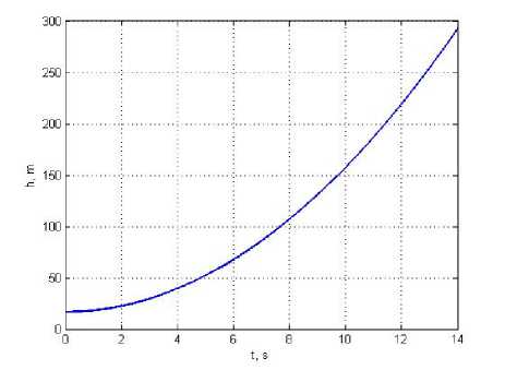
Fig. 3. LV altitude of flight h ( t )

Рис. 3. Высоты полета ЦМ РН

Fig. 7 demonstrates the LV CS regulator coefficients. Fig. 8 shows, that sustainer engine nozzle deviation angle does not exceed 2.5 degrees. After start LV control system commands to deviate the combustion chamber and to hold the current position of LV jet flame on the preset trajectory on starting plane. At 20–30 meters altitude there is some deviation of executed location of LV jet flame from preset location because LV CS provides conditions for further pitch program executing.

Fig. 9 presents the executed and preset positions of LV jet flame trace on the starting plane.

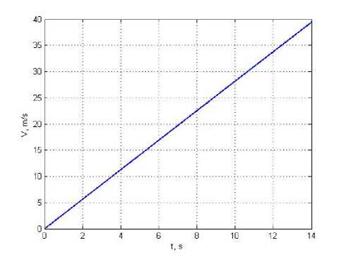
Fig. 4. LV velocity of flight V ( t )

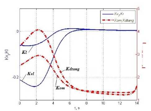
Fig. 7. LV CS regulator coefficients

Рис. 4. Скорость ЦМ РН

Рис. 7. Коэффициенты регулятора СУ РН

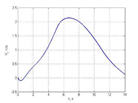
Fig. 5. LV horizontal speed V l ( t )

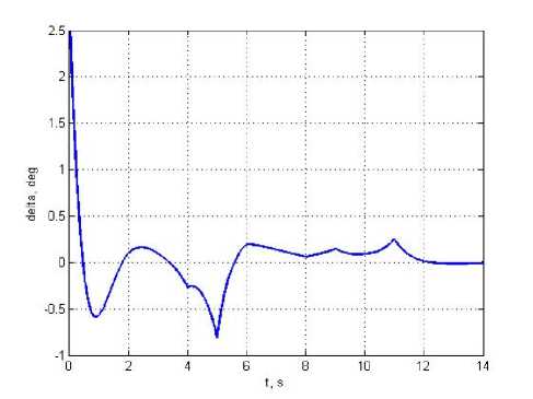
Fig. 8. LV sustainer engine nozzle deviation angle δ ( t )

Рис. 5. Горизонтальная скорость ЦМ РН

Рис. 8. Угол отклонения сопла МД РН

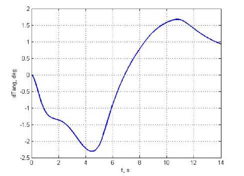
Fig. 6. Increments of LV pitch angle ϑ ( t )

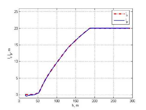
Fig. 9. Preset and executed positions of LV jet flame trace on the starting plane

Рис. 6. Приращение угла тангажа РН

Рис. 9. Заданное и текущее положения следов струи РН на стартовой плоскости

Fig. 10 show that tracking error does not exceed 0.5 meter. It proves the efficiency of developed algorithms for LV controlled motion displace jet flame from starting complex facilities with tolerated accuracy.

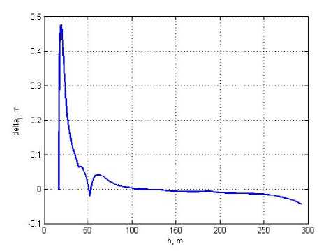
Fig. 10. The difference between preset and executed positions of LV jet flame trace on the starting plane

Рис. 10. Величина рассогласования между заданным и текущим положениями следов струи РН на стартовой плоскости

Conclusion. Having solved problem ACOR for the system (9), (10) with quadratic terminal integral criteria (11), the optimal control of linear nonstationary dynamic system was developed. Dependency of system output vector on input variable was taken into account in optimal control algorithm (22). The solution is valid for the task of displacement of LV jet flame from the starting complex facilities during the preset displacement program execution. It is demonstrated that the optimal regulator (26) and the calculated coefficients (25) satisfy the specified LV CS requirements. It means that the deviations of executed positions of LV jet flame from preset ones does not exceed 0.5 meter. The CS at the end of the displacement maneuver is holding the LV trajectory close to vertical. The value of sustainer engine chamber deviations do not exceed permissible limits and stays in ±2.5 degree interval.

The problem solved is worth to continue by analysis of three-dimensional path of LV and by the LV jet flame trace preset program tacking accuracy analysis taking into account horizontal wind in atmosphere as a random function of altitude using methods of statistical dynamics [15; 16].